

I statistically analyzed the most recent SSC survey. Here is a summary of my results:
People who think the blog got worse are more right wing and less satisfied with their lives. They also have higher SAT scores, but I think that’s due to a collider effect.
ADHD symptoms positively predict self-reported physical attractiveness, but autism symptoms negatively predict it. I have no idea why this is - it could be cross-trait assortative mating or a reporting bias.
Self-reported attractiveness seems to be somewhat valid in this survey - it negatively correlates with BMI (r = -.43 in women, r = -.29 in men) and it’s weakly associated with psychological traits.
Eugenics supporters tend to have higher SAT scores, higher levels of self-reported attractiveness, lower BMIs, lower levels of religiosity, and lower levels of political extremism. Women do not like eugenics, but trans people and men are ok with them.
In terms of international differences, Americans are more right wing and have more symptoms of psychopathological disorders in comparison to Europeans. Slavs like eugenics.
Bisexuals have unusually hypermobile joints, even after controlling for gender. Psychopathological symptoms and joint hypermobility correlated (r = .16), and it doesn’t appear to matter whether self-reports of a diagnosis or the beighton scale itself are used.
Notes:
The composite right wing scale is the first principal component of 14 political questions that were asked.
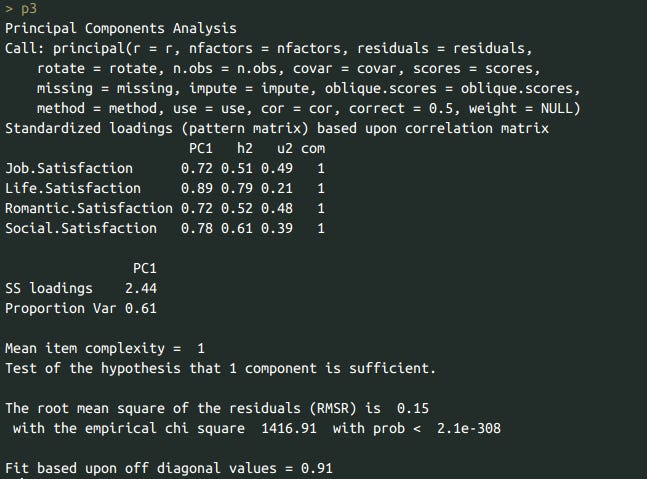
“Satisfaction” is the first principal component of job satisfaction, life satisfaction, romantic satisfaction, and social satisfaction. Omega reliability of 0.83.
Psychopathology a composite of two composites of psychiatric symptoms that use different methodologies. The first is the first principal component of reported psychological disorders, 1-10 anxiety scale, and 1-10 mood scale. The second is a composite which uses an IRT graded unidimensional model that uses scores from the empirical distribution.
Psychopathology had an omega reliability of 0.72. For each disorder, no family history was coded as 0, family history was coded as 1, self-reported diagnosis was coded as 2, diagnosis was coded as 3.
All political questions are coded this way: more right wing → higher value. Supporting eugenics (1-10 scale), being cautious about building housing, and thinking AI is not a problem were coded as right wing. Omega reliability of 0.85.
Part 1: Who thinks the blog got worse?
Right wingers tend to think the blog got worse (rightwing is coded as higher value → more right wing, blogworse is coded as higher value → blog got better).

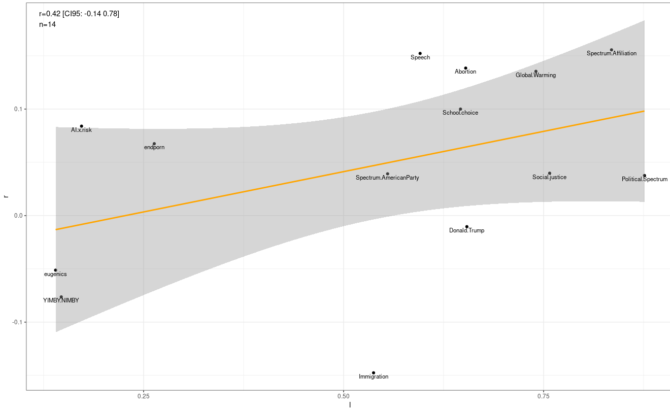
To test for Jensen effects, I plotted the relationship between the correlations each belief (higher value → more right wing) had with believing the blog got worse and the loading each belief had on the first principal component of political beliefs (higher loading → stronger correlation with right wing views). There was a negative correlation, though it’s possible that it was a fluke.

In terms of specific beliefs - the pro eugenics, anti social justice, pro free speech, and global warming skeptic right thinks Scott Alexander’s blog got worse. The others are somewhat more divided.
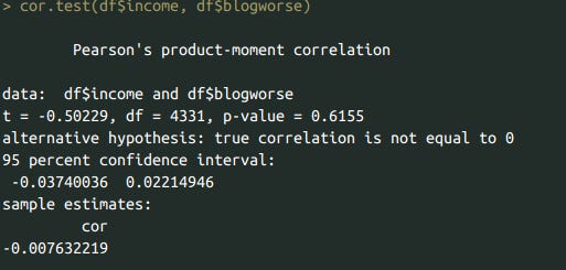
There was no correlation between income and thinking the blog got worse.
People with higher SAT scores think the blog got worse, which is probably due to a collider effect. People who are responding to the survey are people who like the blog and are high in IQ, so within the subsample intelligent people will be more likely to dislike the blog.

No meaningful association with psychopathology.

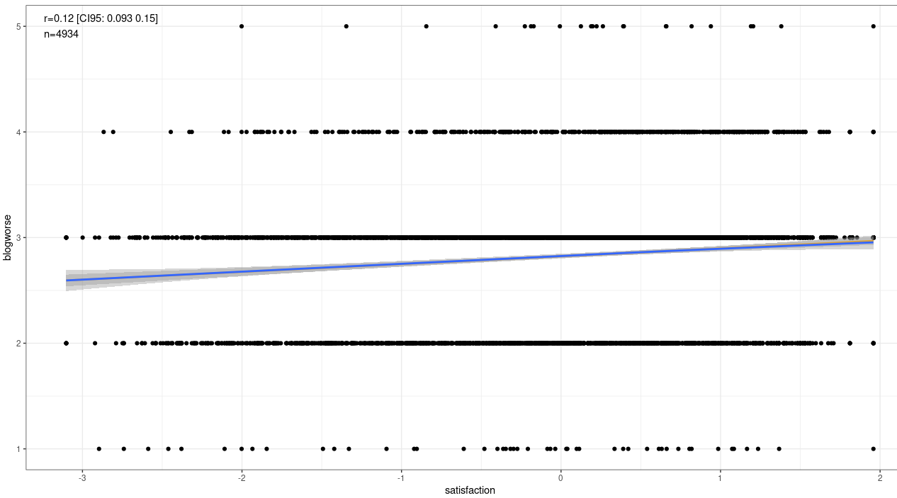
Satisfied people were less likely to think the blog got worse.
Part 2: Physical Attractiveness
I think that physical attractiveness and personality correlate very weakly, and the small observed correlations are due to cross-trait assortative mating, reverse causation (e.g. extraversion causing grooming and grooming causing physical attractiveness), and/or confounding with mutational load. Even for traits that theoretically should be affected by attractiveness like confidence, there is no correlation between objective attractiveness and confidence, but there is a correlation between self-reported attractiveness and confidence.
I tested whether reports of psychiatric diagnosis (using the 0-3 scale I made) predicted self-reported attractiveness independent of others using bayesian model averaging. This technique selects the best models from a large set of linear regression models and estimates the probability that a variable has a true association with the dependent variable in an ideal model. The posterior inclusion probability (PIP) refers to the probability that each variable will be in an ideal true model (anything over 95% is probably trustable), and the expected value (EV) is the expected effect each variable has in an ideal bayesian model.
These were the results:

Autism symptoms negatively predicted self-reported attractiveness, while ADHD symptoms, mood, romantic satisfaction, and social satisfaction all positively predicted self-reported attractiveness. The best model was not highly predictive of self-reported attractiveness (R^2 = .088), especially when you consider that the direction of causality for romantic/social satisfaction is probably from attractiveness → satisfaction.
I tested whether the ADHD/Autism associations were due to demographic confounding. They were not.

I also did a second round of bayesian model averaging that combined the robust psychiatric predictors and self-reported political views. These were the results (dependent variable is self-reported attractiveness):

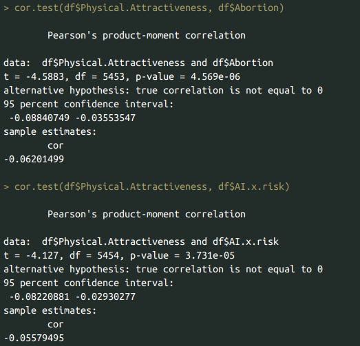
Anti-abortionists and AI risk skeptics had slightly lower levels of attractiveness, eugenics fans and porn haters had slightly higher levels of attractiveness. (Reminder: all political beliefs are coded in a way where higher values correspond to more right wing beliefs). This is corroborated by the zero-order correlations as well.

There is also the question of how valid these ratings are - they’re actually pretty solid. For instance, there is a negative correlation between BMI and self-reported attractiveness (where self-reported attractiveness is controlled for symptoms of autism and ADHD, as well as mood).

The relationship is stronger for women than men.


Interaction test (within cis people only).

The distribution itself is also fairly believable. Very few people gave themselves a 10, and most people gave themselves a 6 or a 7.

Taller people thought they were more attractive, no sex interaction.
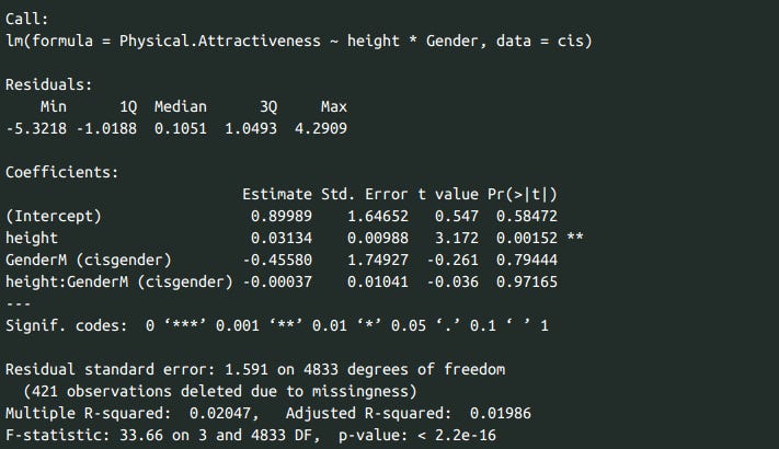

This is roughly what you would expect if there is cross-trait assortative mating between height and attractiveness, as well as some height → attractiveness causation. I suspect that most of the observed correlation is due to environmental factors and cross-trait assortative mating.
Part 3: Who likes eugenics?


Most of the participants were favourable towards eugenics. The scale is valid - on average people who said they supported eugenics were more likely to have said they did on the scale.


There is still some inconsistency between the three metrics, so I increased the validity of attitudes towards eugenics by creating a composite measurement of pro-eugenic beliefs called ‘neoeugenix’ based on the answers to these three questions. It had an omega reliability of .82.
Self-reported attractiveness correlated with endorsement of eugenics.

Political extremists do not like eugenics (note: this measurement of right wing beliefs excluded the measurement of liking eugenics).

ANOVA test between the nonlinear and linear models:

Support for eugenics had a linear and negative association with political interest. I thought for sure that the supporters and opponents of eugenics would be higher in political interest - but I guess I was wrong.

People with higher SAT scores like eugenics more.

Thinner people like eugenics more. Another completely linear association.

Weak correlation between income and support for eugenics.

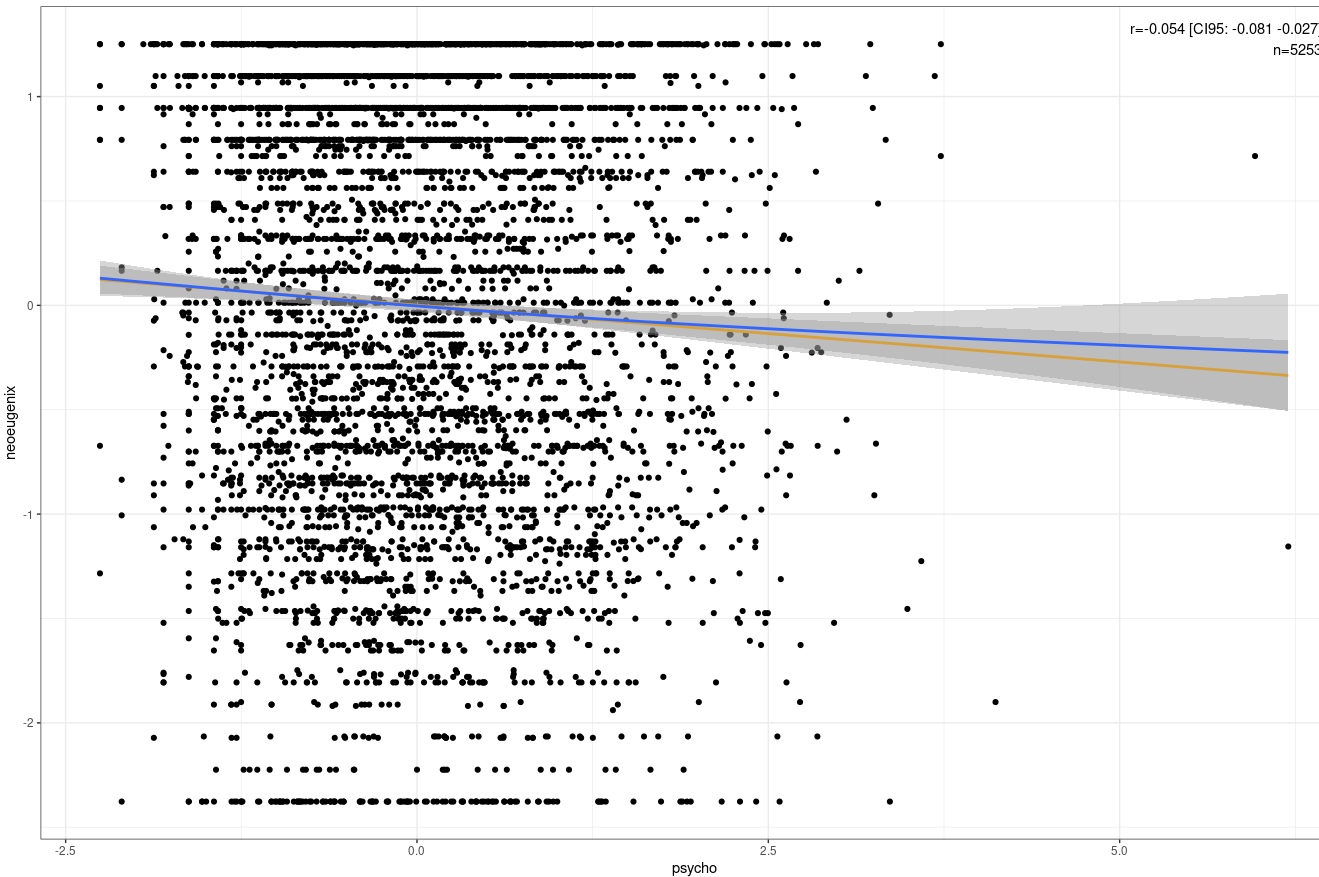
Correlation between support for eugenics and psychopathology. Looks linear, but weak.
Slightly negative (?????) correlation between support for eugenics and overall satisfaction with life.

Negligble correlation between height and support for eugenics. It also disappears when controlling for sex. No interaction either (only cis in this analysis).


No race differences in support for eugenics.

Gender differences in support for eugenics. Nonresponders and women don’t like them, trans people and men are fine with them.

I find Tukey’s posthoc tests to be unnecessary in most cases, but in this situation they should do fine. The difference between cis men and trans people (both FtM and MtF) doesn’t pass significance.

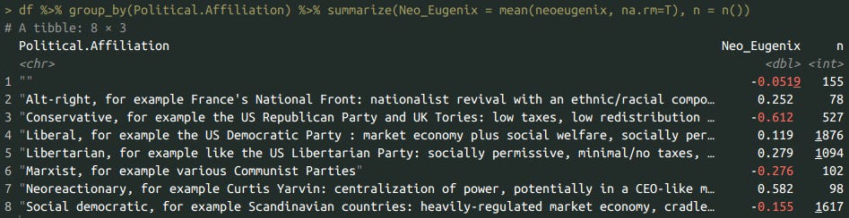
Support for eugenics by political affiliation. Conservatives like eugenics even less than Marxists do.
ANOVA test:

Support by religious views. Committed theists are a full standard deviation below the whole sample in support for eugenics.

ANOVA test:
Tried the BMA method to test the association between specific psychopathologies and support for eugenics. ADHD/autism types like eugenics, anxiety/PTSD types don’t. These symptoms generally not predictive of support for eugenics.

To test whether confounding between predictors was an issue, I used a BMA model to test the association between support for eugenics and predictors that worked well at the zero order level, or that I was curious about for other reasons. Higher levels of religiosity predicted opposing eugenics. High SAT scores, self-reported attractiveness, mental stability, and income all predicted support for eugenics.

Admittedly, religiosity is doing a lot of the heavy lifting in terms of explained variance. Dropping it from the model reduces the explained variance by 84% (R^2 = .23 in the original model, R^2 = .036 in the one without religiosity).

I also tested what political views phenotype predicted support for eugenics. Eugenics supporters like school choice, building housing, legal abortion, donald trump, free speech, the existence of pornography, and think that AI risk is real. Large R^2 (.24), which is driven by views on abortion (standardized beta = -.38) and disliking social justice (standardized beta = .21). The other beliefs are not so predictive.

Part 4: political views and psychopathology.
Right wingers had higher levels of mental stability than left wingers. No nonlinear association detected.

When the chart is rotated the other way around, there is a slight nonlinear association where extremely left wing have disproportionately high levels of psychopathology.

ANOVA test:

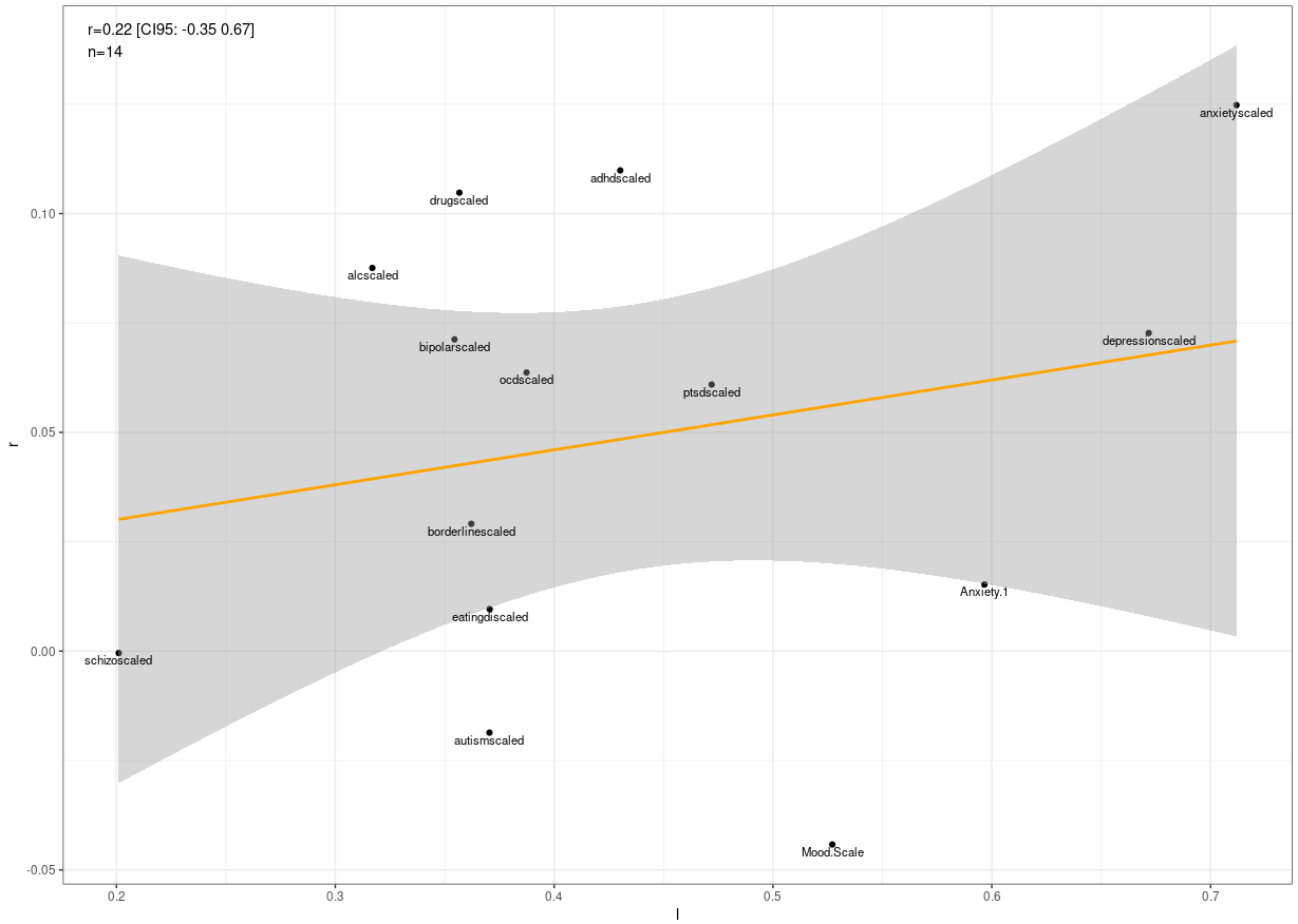
I tried the method of correlated vectors in both directions. In both cases, it suggested that this association was on the general factor of both variables.


Part 5: international differences
As a sanity test, I’ll try computing an obvious one (BMI). Anglos are fatter than the Europeans, which checks out with measured data as well.


Now I’ll try psychopathology.

ANOVA test:

Americans were unusually mentally ill in comparison to Europeans. I formally tested this theory by coding Americans as 1 and Europeans as 0 in my ‘burger’ variable, and found that Americans were 0.25 SD more psychopathological than Europeans.

I tested whether this association was on the general factor using the method of correlated factors, and found that it probably isn’t. Notably, Americans are more likely to report anxiety diagnosis/symptoms/family history, but this is much less true when they are asked about their symptoms on a 1-10 scale (r = .01, p = .30), so there must be some bias that occurs due to using certain measurements over others.
These are the differences in overall life satisfaction:

Indians and Russians seem a bit dissatisifed. The diferences in most countries are fairly small. ANOVA p-value = .0019.
These are the differences in support for eugenics:


Slavs seem to like eugenics, which passes significance when doing a regional comparison.

Lastly, I tested country differences in political views. Americans are more right wing than Europeans.

ANOVA test:
Using the same methodology that was used to test American vs European differences in psychopathology, I found that Americans were 0.21 SD more right wing than Europeans.

There was no clear Jensen effect. Americans had more right wing views on free speech, abortion, and global warming; but more left wing views on eugenics, building housing, and immigration.
Part 6: strechy joints
There is some literature and reviews that suggest that people with hypermobile joints are psychologically strange. Scott Alexander included one self-report and one scale.


The self-reports look accurate.

I combined the measurements, but I gave twice the weight to the scale, and normalized it to mean = 0 and SD = 1. I found a robust correlation between psychopathology and hypermobility.
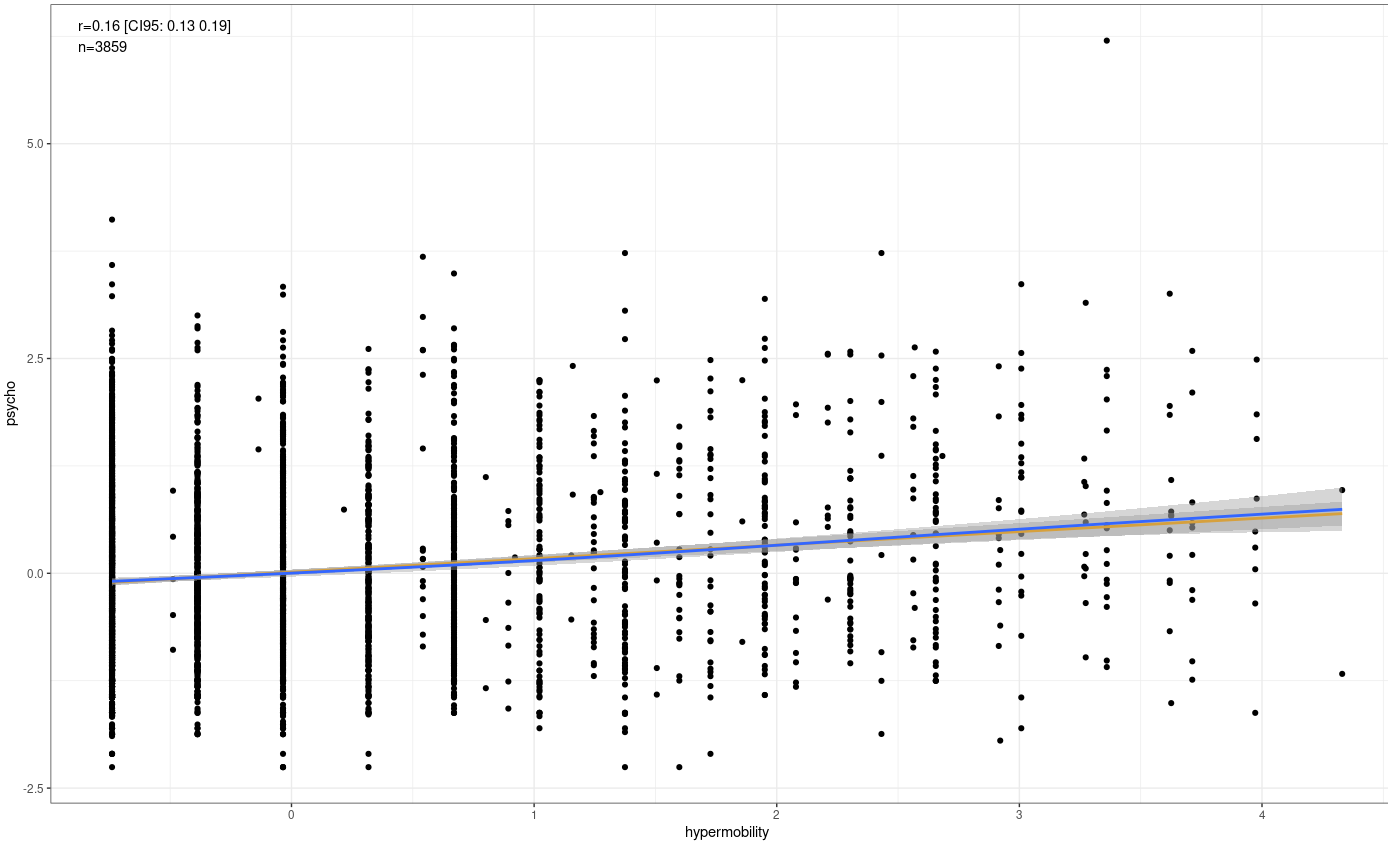
This was true regardless of whether the beighton (for some reason, my eyes read it as breighton) scale was used, or whether the self-reported scale was used (superscale).

Trans women had more hypermobile joints than cis men, and trans men had more hypermobile joints than cis women. I then tested for biological male and trans specific effects, and found a biological male effect (d = -.50) and trans effect (d = .28). No interaction between biological sex and being trans was detected.


Bisexuals and homosexuals had more hypermobile joints than heterosexuals.

To avoid cofounding with gender, I controlled the hypermobility measurement for gender. Differences are smaller, but still persistent - particularly for bisexuals.

I pulled out the bayesian model averaging again to test whether specific psychiatric symptoms are responsible for this association, and found that autism and anxiety in particular were predictive of joint hypermobility, even when gender identity is controlled for.

No idea if it’s a Jensen effect.

Appendix
Reliabilities of composite variables:


PCA results for political beliefs:

PCA results for psychopathology symptoms:

IRT model of psychopathology symptoms:

PCA results for satisfaction:
Sanity tests:
Right wing beliefs by gender. Trans people are -0.75 SD below cis men, and women are 0.3 SD below cis men.

No race differences in political beliefs.

Code (note: I used several personal functions and libraries that most people do not have access to):
df <- tljensen
colnames(df)

df %>% group_by(What.are.your.thoughts.on.polygenic.selection.against.disease.) %>% summarize(Right = mean(Political.Spectrum, na.rm=T))
df %>% group_by(Political.Affiliation) %>% summarize(Right = mean(Political.Spectrum, na.rm=T))

df$SATM <- as.numeric(df$SAT.score.math)
df$SATV <- as.numeric(df$SAT.score.verbal.reading)
df$SATV[df$SATV > 800] <- NA
df$SATV[df$SATV < 200] <- NA
df$SATM[df$SATM > 800] <- NA
df$SATM[df$SATM < 200] <- NA
df$SAT <- df$SATM + df$SATV
df$SAT[df$SAT > 1600] <- NA
df$SAT[df$SAT < 400] <- NA

df$BMI <- as.numeric(df$What.is.your.BMI.)
df$BMI[df$BMI > 50] <- NA
df$BMI[df$BMI < 12] <- NA

df$height <- as.numeric(df$What.is.your.height.in.centimeters.)
df$height[df$height > 250] <- NA
df$height[df$height < 100] <- NA

df$Spectrum.Affiliation <- NA
df$Spectrum.AmericanParty <- NA
df$Spectrum.AmericanParty[df$American.Parties=='Democratic Party'] <- 3.59
df$Spectrum.AmericanParty[df$American.Parties=='Republican Party'] <- 7.02
df$Spectrum.AmericanParty[df$American.Parties=='Libertarian Party'] <- 6.08
df$Spectrum.AmericanParty[df$American.Parties==''] <- 4.6
df$Spectrum.AmericanParty[df$American.Parties=='(option for non-Americans who want an option)'] <- 4.63
df$Spectrum.AmericanParty[df$American.Parties=='Not registered for a party'] <- 5.11
df$Spectrum.AmericanParty[df$American.Parties=='Other third party'] <- 4.5

df$Spectrum.Affiliation[grepl("Marxist, for example various Communist Parties", df$Political.Affiliation, fixed=TRUE)] <- 1.83
df$Spectrum.Affiliation[grepl("Social democratic, for example Scandinavian countries: heavily-regulated market economy, cradle-to-grave social safety net, socially permissive multiculturalism", df$Political.Affiliation, fixed=TRUE)] <-3.28
df$Spectrum.Affiliation[grepl("Liberal, for example the US Democratic Party : market economy plus social welfare, socially permissive multiculturalism", df$Political.Affiliation, fixed=TRUE)] <- 4.09
df$Spectrum.Affiliation[grepl("Libertarian, for example like the US Libertarian Party: socially permissive, minimal/no taxes, minimal/no distribution of wealth", df$Political.Affiliation, fixed=TRUE)] <- 6.08
df$Spectrum.Affiliation[grepl("Conservative, for example the US Republican Party and UK Tories: low taxes, low redistribution of wealth,  traditional values", df$Political.Affiliation, fixed=TRUE)] <- 7.18
df$Spectrum.Affiliation[grepl("Neoreactionary, for example Curtis Yarvin: centralization of power, potentially in a CEO-like monarch, is necessary for good government", df$Political.Affiliation, fixed=TRUE)] <- 7.82
df$Spectrum.Affiliation[grepl("Alt-right, for example France's National Front: nationalist revival with an ethnic/racial component", df$Political.Affiliation, fixed=TRUE)] <-8.13
df$Spectrum.Affiliation[df$Political.Affiliation==''] <- 5.15

df$endporn <- NA
df$endporn[df$End.all.porn=='Yes'] <- 1
df$endporn[df$End.all.porn=='No'] <- 0

df$Immigration <- -df$Immigration
df$Speech <- -df$Speech
df$YIMBY.NIMBY <- -df$YIMBY.NIMBY
df$Social.justice <- -df$Social.justice
df$Abortion <- -df$Abortion
df$AI.x.risk <- -df$AI.x.risk
df$eugenics <- df$How.do.you.feel.about.non.coercive.eugenics.

df$rightwing <- getpc(df %>% select(Political.Spectrum, Spectrum.Affiliation, Global.Warming, Spectrum.AmericanParty, Immigration, School.choice, YIMBY.NIMBY, Social.justice, Abortion, Donald.Trump, Speech, AI.x.risk, endporn, eugenics), dofa=F, normalizeit=T)
df$blogworse <- df$Has.the.blog.gotten.better.or.worse.since.you.started.reading.it.

cor.test(df$rightwing, df$blogworse)

p <- pca(df %>% select(Political.Spectrum, Spectrum.Affiliation, Global.Warming, Spectrum.AmericanParty, Immigration, School.choice, YIMBY.NIMBY, Social.justice, Abortion, Donald.Trump, Speech, AI.x.risk, endporn, eugenics), rotate='none', nfactors=1)
p
debi <- data.frame(v = rep('', 14), r = rep(0, 14))
debi$v <- NA
i = 1
for(vec in c('Political.Spectrum', 'Spectrum.Affiliation', 'Global.Warming', 'Spectrum.AmericanParty', 'Immigration', 'School.choice', 'YIMBY.NIMBY', 'Social.justice', 'Abortion', 'Donald.Trump', 'Speech', 'AI.x.risk', 'endporn', 'eugenics')) {
  debi$v[i] <- vec
  debi$r[i] <- cor.test(df[[vec]], df$blogworse)$estimate
  i = i + 1
}
debi$v
debi$l <- p$loadings
GG_scatter(df=debi, x_var='l', y_var='r', case_names = 'v')

################
df$income <- as.numeric(df$Income)
cor.test(df$income, df$blogworse)
cor.test(df$SAT, df$blogworse)

#################
df$depressionscaled[df$Depression=="I don't have this condition and neither does anyone in my family"] <- 0
df$depressionscaled[df$Depression=="I have family members (within two generations) with this condition"] <- 1
df$depressionscaled[df$Depression=="I think I might have this condition, although I have never been formally diagnosed"] <- 2
df$depressionscaled[df$Depression=="I have a formal diagnosis of this condition"] <- 3

df$anxietyscaled[df$Anxiety=="I don't have this condition and neither does anyone in my family"] <- 0
df$anxietyscaled[df$Anxiety=="I have family members (within two generations) with this condition"] <- 1
df$anxietyscaled[df$Anxiety=="I think I might have this condition, although I have never been formally diagnosed"] <- 2
df$anxietyscaled[df$Anxiety=="I have a formal diagnosis of this condition"] <- 3

df$ocdscaled[df$OCD=="I don't have this condition and neither does anyone in my family"] <- 0
df$ocdscaled[df$OCD=="I have family members (within two generations) with this condition"] <- 1
df$ocdscaled[df$OCD=="I think I might have this condition, although I have never been formally diagnosed"] <- 2
df$ocdscaled[df$OCD=="I have a formal diagnosis of this condition"] <- 3

df$eatingdiscaled[df$Eating.disorder=="I don't have this condition and neither does anyone in my family"] <- 0
df$eatingdiscaled[df$Eating.disorder=="I have family members (within two generations) with this condition"] <- 1
df$eatingdiscaled[df$Eating.disorder=="I think I might have this condition, although I have never been formally diagnosed"] <- 2
df$eatingdiscaled[df$Eating.disorder=="I have a formal diagnosis of this condition"] <- 3

df$ptsdscaled[df$PTSD=="I don't have this condition and neither does anyone in my family"] <- 0
df$ptsdscaled[df$PTSD=="I have family members (within two generations) with this condition"] <- 1
df$ptsdscaled[df$PTSD=="I think I might have this condition, although I have never been formally diagnosed"] <- 2
df$ptsdscaled[df$PTSD=="I have a formal diagnosis of this condition"] <- 3

df$alcscaled[df$Alcoholism=="I don't have this condition and neither does anyone in my family"] <- 0
df$alcscaled[df$Alcoholism=="I have family members (within two generations) with this condition"] <- 1
df$alcscaled[df$Alcoholism=="I think I might have this condition, although I have never been formally diagnosed"] <- 2
df$alcscaled[df$Alcoholism=="I have a formal diagnosis of this condition"] <- 3

df$drugscaled[df$Drug.addiction=="I don't have this condition and neither does anyone in my family"] <- 0
df$drugscaled[df$Drug.addiction=="I have family members (within two generations) with this condition"] <- 1
df$drugscaled[df$Drug.addiction=="I think I might have this condition, although I have never been formally diagnosed"] <- 2
df$drugscaled[df$Drug.addiction=="I have a formal diagnosis of this condition"] <- 3

df$borderlinescaled[df$Borderline=="I don't have this condition and neither does anyone in my family"] <- 0
df$borderlinescaled[df$Borderline=="I have family members (within two generations) with this condition"] <- 1
df$borderlinescaled[df$Borderline=="I think I might have this condition, although I have never been formally diagnosed"] <- 2
df$borderlinescaled[df$Borderline=="I have a formal diagnosis of this condition"] <- 3

df$bipolarscaled[df$Bipolar=="I don't have this condition and neither does anyone in my family"] <- 0
df$bipolarscaled[df$Bipolar=="I have family members (within two generations) with this condition"] <- 1
df$bipolarscaled[df$Bipolar=="I think I might have this condition, although I have never been formally diagnosed"] <- 2
df$bipolarscaled[df$Bipolar=="I have a formal diagnosis of this condition"] <- 3

df$autismscaled[df$Autism=="I don't have this condition and neither does anyone in my family"] <- 0
df$autismscaled[df$Autism=="I have family members (within two generations) with this condition"] <- 1
df$autismscaled[df$Autism=="I think I might have this condition, although I have never been formally diagnosed"] <- 2
df$autismscaled[df$Autism=="I have a formal diagnosis of this condition"] <- 3

df$adhdscaled[df$ADHD=="I don't have this condition and neither does anyone in my family"] <- 0
df$adhdscaled[df$ADHD=="I have family members (within two generations) with this condition"] <- 1
df$adhdscaled[df$ADHD=="I think I might have this condition, although I have never been formally diagnosed"] <- 2
df$adhdscaled[df$ADHD=="I have a formal diagnosis of this condition"] <- 3

df$schizoscaled[df$Schizophrenia=="I don't have this condition and neither does anyone in my family"] <- 0
df$schizoscaled[df$Schizophrenia=="I have family members (within two generations) with this condition"] <- 1
df$schizoscaled[df$Schizophrenia=="I think I might have this condition, although I have never been formally diagnosed"] <- 2
df$schizoscaled[df$Schizophrenia=="I have a formal diagnosis of this condition"] <- 3
df$psychopathology <- getpc(df %>% select(schizoscaled, autismscaled, adhdscaled, bipolarscaled, borderlinescaled, drugscaled, alcscaled, ptsdscaled, eatingdiscaled, ocdscaled, anxietyscaled, depressionscaled, Anxiety.1, Mood.Scale), normalizeit = T, fillmissing = T, dofa=F)
df$satisfaction <- getpc(df %>% select(Job.Satisfaction, Life.Satisfaction, Romantic.Satisfaction, Social.Satisfaction), normalizeit = T, fillmissing = F, dofa=F)
df$drugscaled[191] <- 0


m <- mirt(df %>% select(schizoscaled, autismscaled, adhdscaled, bipolarscaled, borderlinescaled, drugscaled, alcscaled, ptsdscaled, eatingdiscaled, ocdscaled, anxietyscaled, depressionscaled, Anxiety.1, Mood.Scale), model=1, graded=T, dentype='empiricalhist')
summary(m)

adele <- fscores(m, full.scores = TRUE, full.scores.SE=T)
adele2 <- fscores(m, full.scores = TRUE)
empirical_rxx(adele)
df$psychopathologyirt <- adele2
df$psycho <- normalise(normalise(df$psychopathologyirt) + normalise(df$psychopathology))

describe2(df$psycho)
describe2(df$rightwing)

p2 <- pca(df %>% select(schizoscaled, autismscaled, adhdscaled, bipolarscaled, borderlinescaled, drugscaled, alcscaled, ptsdscaled, eatingdiscaled, ocdscaled, anxietyscaled, depressionscaled, Anxiety.1, Mood.Scale), rotate='none', nfactors=1)
p2

p3 <- pca(df %>% select(Job.Satisfaction, Life.Satisfaction, Romantic.Satisfaction, Social.Satisfaction), rotate='none', nfactors=1)
p3

cor.test(df$psychopathology, df$satisfaction)
cor.test(df$rightwing, df$satisfaction)

cor.test(df$psychopathology, df$rightwing)
cor.test(df$satisfaction, df$rightwing)


########
GG_scatter(df, x_var='rightwing', y_var='blogworse') + geom_smooth()

GG_scatter(df, x_var='psycho', y_var='blogworse') + geom_smooth()
GG_scatter(df, x_var='satisfaction', y_var='blogworse') + geom_smooth()

GG_denhist(df$BMI)


###########
reliability(df %>% select(Job.Satisfaction, Life.Satisfaction, Romantic.Satisfaction, Social.Satisfaction))
reliability(df %>% select(schizoscaled, autismscaled, adhdscaled, bipolarscaled, borderlinescaled, drugscaled, alcscaled, ptsdscaled, eatingdiscaled, ocdscaled, anxietyscaled, depressionscaled, Anxiety.1, Mood.Scale))
reliability(df %>% select(Political.Spectrum, Spectrum.Affiliation, Global.Warming, Spectrum.AmericanParty, Immigration, School.choice, YIMBY.NIMBY, Social.justice, Abortion, Donald.Trump, Speech, AI.x.risk, endporn, eugenics))

quantile(df$rightwing, probs=seq(0, 1, 0.01), na.rm=T)

###############################
ind <- subset(df, select=c('schizoscaled', 'autismscaled', 'adhdscaled', 'bipolarscaled', 'borderlinescaled', 'drugscaled', 'alcscaled', 'ptsdscaled', 'eatingdiscaled', 'ocdscaled', 'anxietyscaled', 'depressionscaled', 'Anxiety.1', 'Mood.Scale', 'Job.Satisfaction', 'Life.Satisfaction', 'Romantic.Satisfaction', 'Social.Satisfaction', 'Physical.Attractiveness'))
ind <- na.omit(ind)
nrow(ind)

names <- c('schizoscaled', 'autismscaled', 'adhdscaled', 'bipolarscaled', 'borderlinescaled', 'drugscaled', 'alcscaled', 'ptsdscaled', 'eatingdiscaled', 'ocdscaled', 'anxietyscaled', 'depressionscaled', 'Anxiety.1', 'Mood.Scale', 'Job.Satisfaction', 'Life.Satisfaction', 'Romantic.Satisfaction', 'Social.Satisfaction', 'Physical.Attractiveness')
nrow(ind)
for(name in names) {
  ind[[name]] = normalise(ind[[name]])
}

bmalol <- bicreg(x = ind %>% select(-Physical.Attractiveness), y = ind$Physical.Attractiveness, maxCol=999, nbest=999, OR=20, strict=FALSE)
summary(bmalol)

lr <- lm(data=df, Physical.Attractiveness ~ autismscaled + adhdscaled + as.factor(Gender) + as.factor(Race) + as.factor(Age) + as.factor(Sexual.Orientation))
summary(lr)
############################
ind <- subset(df, select=c('autismscaled', 'adhdscaled', 'Mood.Scale', 'Romantic.Satisfaction', 'Social.Satisfaction', 'Physical.Attractiveness', 'rightwing', 'Global.Warming', 'Immigration', 'School.choice', 'YIMBY.NIMBY', 'Social.justice', 'Abortion', 'Donald.Trump', 'Speech', 'AI.x.risk', 'endporn', 'eugenics'))
ind <- na.omit(ind)
nrow(ind)

names <- c('autismscaled', 'adhdscaled', 'Mood.Scale', 'Romantic.Satisfaction', 'Social.Satisfaction', 'Physical.Attractiveness', 'rightwing', 'Global.Warming', 'Immigration', 'School.choice', 'YIMBY.NIMBY', 'Social.justice', 'Abortion', 'Donald.Trump', 'Speech', 'AI.x.risk', 'endporn', 'eugenics')
nrow(ind)
for(name in names) {
  ind[[name]] = normalise(ind[[name]])
}

bmalol <- bicreg(x = ind %>% select(-Physical.Attractiveness), y = ind$Physical.Attractiveness, maxCol=999, nbest=999, OR=20, strict=FALSE)
summary(bmalol)


cor.test(df$Physical.Attractiveness, df$Abortion)
cor.test(df$Physical.Attractiveness, df$AI.x.risk)
cor.test(df$Physical.Attractiveness, df$endporn)
cor.test(df$Physical.Attractiveness, df$eugenics)
cor.test(df$Physical.Attractiveness, df$psycho)

GG_scatter(df, 'BMI', 'Physical.Attractiveness') + geom_smooth()
################
cor.test(df$Physical.Attractiveness, df$psycho)
cor.test(df$Physical.Attractiveness, df$autismscaled)

lr <- lm(data=df, Physical.Attractiveness ~ autismscaled + adhdscaled + Mood.Scale)
summary(lr)

df$residualattractiveness[!is.na(df$autismscaled) & !is.na(df$adhdscaled) & !is.na(df$Mood.Scale) & !is.na(df$Physical.Attractiveness)] <- normalise(lr$residuals)

##################
cor.test(df$residualattractiveness, df$Physical.Attractiveness)

GG_scatter(df, 'BMI', 'residualattractiveness') + geom_smooth()

GG_scatter(df, 'BMI', 'Physical.Attractiveness') + geom_smooth()

female <- df %>% filter(Gender=='F (cisgender)')
male <- df %>% filter(Gender=='M (cisgender)')

GG_scatter(female, 'BMI', 'residualattractiveness') + geom_smooth() + labs(title='Women only')
GG_scatter(male, 'BMI', 'residualattractiveness') + geom_smooth() + labs(title='Men only')

cis <- df %>% filter(Gender=='M (cisgender)' | Gender=='F (cisgender)')

lr <- lm(data=cis, residualattractiveness ~ BMI*Gender)
summary(lr)

###########################
df %>% group_by(What.are.your.thoughts.on.polygenic.selection.against.disease.) %>% summarize(eugenics = mean(eugenics, na.rm=T), n = n())
df %>% group_by(What.are.your.thoughts.on.polygenic.selection.for.cognitive.physical.traits.) %>% summarize(eugenics = mean(eugenics, na.rm=T), n = n())

df$bioeugenics <- NA
df$bioeugenics[df$What.are.your.thoughts.on.polygenic.selection.for.cognitive.physical.traits.==''] <- 5.03
df$bioeugenics[df$What.are.your.thoughts.on.polygenic.selection.for.cognitive.physical.traits.=='Against it and want it banned'] <- 2.96
df$bioeugenics[df$What.are.your.thoughts.on.polygenic.selection.for.cognitive.physical.traits.=="Don't know what it is, or have no opinion"] <- 4.58
df$bioeugenics[df$What.are.your.thoughts.on.polygenic.selection.for.cognitive.physical.traits.=="In favor of it and have used it (or am in the process of using it)"] <- 7.22
df$bioeugenics[df$What.are.your.thoughts.on.polygenic.selection.for.cognitive.physical.traits.=="In favor of it, and will/would use it if I ever had children via IVF"] <- 7.23
df$bioeugenics[df$What.are.your.thoughts.on.polygenic.selection.for.cognitive.physical.traits.=="In favor of it, but wouldn't want it personally (because of cost, convenience, etc)"] <- 6.55
df$bioeugenics[df$What.are.your.thoughts.on.polygenic.selection.for.cognitive.physical.traits.=="Not against it per se, but skeptical and don't think it's worth it right now"] <- 4.9
df$bioeugenics[df$What.are.your.thoughts.on.polygenic.selection.for.cognitive.physical.traits.=="Personally against it, but don't want it banned"] <- 4.02

df$diseaseeugenics <- NA
df$diseaseeugenics[df$What.are.your.thoughts.on.polygenic.selection.against.disease.==''] <- 5.03
df$diseaseeugenics[df$What.are.your.thoughts.on.polygenic.selection.against.disease.=='Against it and want it banned'] <- 2.96
df$diseaseeugenics[df$What.are.your.thoughts.on.polygenic.selection.against.disease.=="Don't know what it is, or have no opinion"] <- 4.58
df$diseaseeugenics[df$What.are.your.thoughts.on.polygenic.selection.against.disease.=="In favor of it and have used it (or am in the process of using it)"] <- 7.22
df$diseaseeugenics[df$What.are.your.thoughts.on.polygenic.selection.against.disease.=="In favor of it, and will/would use it if I ever had children via IVF"] <- 7.23
df$diseaseeugenics[df$What.are.your.thoughts.on.polygenic.selection.against.disease.=="In favor of it, but wouldn't want it personally (because of cost, convenience, etc)"] <- 6.55
df$diseaseeugenics[df$What.are.your.thoughts.on.polygenic.selection.against.disease.=="Not against it per se, but skeptical and don't think it's worth it right now"] <- 4.9
df$diseaseeugenics[df$What.are.your.thoughts.on.polygenic.selection.against.disease.=="Personally against it, but don't want it banned"] <- 4.02

cor.test(df$diseaseeugenics, df$bioeugenics)
cor.test(df$diseaseeugenics, df$eugenics)
cor.test(df$bioeugenics, df$eugenics)

df$neoeugenix <- getpc(df %>% select(diseaseeugenics, bioeugenics, eugenics), normalizeit = T, fillmissing = F, dofa=F)

print(df %>% group_by(Race) %>% summarise(eugenicsmean = mean(neoeugenix, na.rm=T), n = n()), n=10)
summary(aov(df$neoeugenix ~ df$Race))

print(df %>% group_by(Gender) %>% summarise(eugenicsmean = mean(neoeugenix, na.rm=T), n = n()), n=10)
summary(aov(df$neoeugenix ~ df$Gender))

trans <- aov(df$neoeugenix ~ df$Gender)
tukey_test <- TukeyHSD(trans)
print(tukey_test)

reliability(df %>% select(diseaseeugenics, bioeugenics, eugenics))

GG_scatter(df, 'residualattractiveness', 'neoeugenix')

df$rightwing2 <- getpc(df %>% select(Political.Spectrum, Spectrum.Affiliation, Global.Warming, Spectrum.AmericanParty, Immigration, School.choice, YIMBY.NIMBY, Social.justice, Abortion, Donald.Trump, Speech, AI.x.risk, endporn), dofa=F, normalizeit=T)
print(df %>% group_by(Gender) %>% summarise(rw = mean(rightwing, na.rm=T), n = n()), n=10)
summary(aov(df$rightwing ~ df$Gender))

print(df %>% group_by(Race) %>% summarise(rw = mean(rightwing, na.rm=T), n = n()), n=10)
summary(aov(df$rightwing ~ df$Race))

GG_scatter(df, 'rightwing2', 'neoeugenix') + geom_smooth()

lr <- lm(data=df, neoeugenix ~ rightwing2)
summary(lr)
lr2 <- lm(data=df, neoeugenix ~ rcs(rightwing2, 5))
summary(lr2)

anova(lr, lr2)

GG_scatter(df, 'neoeugenix', 'Political.Interest') + geom_smooth()

GG_scatter(df, 'SAT', 'neoeugenix') + geom_smooth()
cor.test(df$SAT, df$neoeugenix)

GG_scatter(df, 'BMI', 'neoeugenix') + geom_smooth()
cor.test(df$BMI, df$neoeugenix)

GG_scatter(df, 'income', 'neoeugenix') + geom_smooth()
cor.test(df$income, df$neoeugenix)

GG_scatter(df, 'psycho', 'neoeugenix') + geom_smooth()
cor.test(df$psycho, df$neoeugenix)

GG_scatter(df, 'satisfaction', 'neoeugenix') + geom_smooth()
cor.test(df$satisfaction, df$neoeugenix)

GG_scatter(df, 'height', 'neoeugenix') + geom_smooth()
cor.test(df$height, df$neoeugenix)

cis <- df %>% filter(Gender=='M (cisgender)' | Gender=='F (cisgender)')

lr <- lm(data=cis, neoeugenix ~ Gender*height)
summary(lr)

lr <- lm(data=cis, neoeugenix ~ height)
summary(lr)

lr <- lm(data=cis, neoeugenix ~ Gender + height)
summary(lr)

lr <- lm(data=cis, neoeugenix ~ Gender*height)
summary(lr)


df %>% group_by(Political.Affiliation) %>% summarize(Neo_Eugenix = mean(neoeugenix, na.rm=T), n = n())
summary(aov(df$neoeugenix ~ df$Political.Affiliation))

df %>% group_by(Religious.Views) %>% summarize(Neo_Eugenix = mean(neoeugenix, na.rm=T), n = n())
summary(aov(df$neoeugenix ~ df$Religious.Views))

###############################
ind <- subset(df, select=c('schizoscaled', 'autismscaled', 'adhdscaled', 'bipolarscaled', 'borderlinescaled', 'drugscaled', 'alcscaled', 'ptsdscaled', 'eatingdiscaled', 'ocdscaled', 'anxietyscaled', 'depressionscaled', 'Anxiety.1', 'Mood.Scale', 'Job.Satisfaction', 'Life.Satisfaction', 'Romantic.Satisfaction', 'Social.Satisfaction', 'neoeugenix'))
ind <- na.omit(ind)
nrow(ind)

names <- c('schizoscaled', 'autismscaled', 'adhdscaled', 'bipolarscaled', 'borderlinescaled', 'drugscaled', 'alcscaled', 'ptsdscaled', 'eatingdiscaled', 'ocdscaled', 'anxietyscaled', 'depressionscaled', 'Anxiety.1', 'Mood.Scale', 'Job.Satisfaction', 'Life.Satisfaction', 'Romantic.Satisfaction', 'Social.Satisfaction', 'neoeugenix')
nrow(ind)
for(name in names) {
  ind[[name]] = normalise(ind[[name]])

}
bmalol <- bicreg(x = ind %>% select(-neoeugenix), y = ind$neoeugenix, maxCol=999, nbest=999, OR=20, strict=FALSE)
summary(bmalol)
###############################
ind <- subset(df, select=c('psycho', 'SAT', 'BMI', 'residualattractiveness', 'income', 'satisfaction', 'Religious.Views', 'neoeugenix'))
ind <- na.omit(ind)
nrow(ind)

names <- c('psycho', 'SAT', 'BMI', 'residualattractiveness', 'income', 'satisfaction')
nrow(ind)
for(name in names) {
  ind[[name]] = normalise(ind[[name]])
}

bmalol <- bicreg(x = ind %>% select(-neoeugenix, -Religious.Views), y = ind$neoeugenix, maxCol=999, nbest=999, OR=20, strict=FALSE)
summary(bmalol)


###############################
ind <- subset(df, select=c('rightwing2', 'Global.Warming', 'Immigration', 'School.choice', 'YIMBY.NIMBY', 'Social.justice', 'Abortion', 'Donald.Trump', 'Speech', 'AI.x.risk', 'endporn', 'neoeugenix'))
ind <- na.omit(ind)
nrow(ind)

names <- c('rightwing2', 'Global.Warming', 'Immigration', 'School.choice', 'YIMBY.NIMBY', 'Social.justice', 'Abortion', 'Donald.Trump', 'Speech', 'AI.x.risk', 'endporn', 'neoeugenix')
nrow(ind)
for(name in names) {
  ind[[name]] = normalise(ind[[name]])
}

bmalol <- bicreg(x = ind %>% select(-neoeugenix), y = ind$neoeugenix, maxCol=999, nbest=999, OR=20, strict=FALSE)
summary(bmalol)

cor.test(df$eugenics, df$Abortion)


colnames(df)

GG_scatter(df, 'psycho', 'rightwing') + geom_smooth()
GG_scatter(df, 'rightwing', 'psycho') + geom_smooth()

lr <- lm(data=df, psycho ~ rightwing)
summary(lr)
lr2 <- lm(data=df, psycho ~ rcs(rightwing, 5))
summary(lr2)

anova(lr, lr2)
####################################
debi <- data.frame(v = rep('', 14), r = rep(0, 14))
debi$v <- NA
i = 1
for(vec in c('Political.Spectrum', 'Spectrum.Affiliation', 'Global.Warming', 'Spectrum.AmericanParty', 'Immigration', 'School.choice', 'YIMBY.NIMBY', 'Social.justice', 'Abortion', 'Donald.Trump', 'Speech', 'AI.x.risk', 'endporn', 'eugenics')) {
  debi$v[i] <- vec
  debi$r[i] <- cor.test(df[[vec]], df$psycho)$estimate
  i = i + 1
}
debi$v
debi$l <- p$loadings
GG_scatter(df=debi, x_var='l', y_var='r', case_names = 'v')

###########33
debi <- data.frame(v = rep('', 14), r = rep(0, 14))
debi$v <- NA
i = 1
for(vec in c('schizoscaled', 'autismscaled', 'adhdscaled', 'bipolarscaled', 'borderlinescaled', 'drugscaled', 'alcscaled', 'ptsdscaled', 'eatingdiscaled', 'ocdscaled', 'anxietyscaled', 'depressionscaled', 'Anxiety.1', 'Mood.Scale')) {
  debi$v[i] <- vec
  debi$r[i] <- cor.test(df[[vec]], df$rightwing)$estimate
  i = i + 1
}
debi$v
debi$l <- p2$loadings
debi$r[14] <- -0.0511642055
debi$l[14] <- 0.5271236
GG_scatter(df=debi, x_var='l', y_var='r', case_names = 'v')


############################
print(df %>% group_by(Country) %>% summarize(mBMI = mean(BMI, na.rm=T), n = n()) %>% arrange(-n), n=50)

summary(aov(df$BMI ~ df$Country))
colnames(df)

print(df %>% group_by(Country) %>% summarize(psycho = mean(psycho, na.rm=T), n = n()) %>% arrange(-n), n=50)

summary(aov(df$psycho ~ df$Country))

df$code <- countrycode(df$Country, origin='country.name', destination='iso3c')
df$code[df$Country==', Swtizerland'] <- 'CHE'

df$cont <- countrycode(df$Country, origin='country.name', destination='continent')
df$cont[df$Country==', Swtizerland'] <- 'Europe'
df$cont
df$burger <- NA
df$burger[df$Country=='United States'] <- 1
df$burger[df$cont=='Europe'] <- 0

cohen.d(data=df, psycho ~ burger)

cohen.d(data=df, psycho ~ burger)$p

debi <- data.frame(v = rep('', 14), r = rep(0, 14))
debi$v <- NA
i = 1
for(vec in c('schizoscaled', 'autismscaled', 'adhdscaled', 'bipolarscaled', 'borderlinescaled', 'drugscaled', 'alcscaled', 'ptsdscaled', 'eatingdiscaled', 'ocdscaled', 'anxietyscaled', 'depressionscaled', 'Anxiety.1', 'Mood.Scale')) {
  debi$v[i] <- vec
  debi$r[i] <- cor.test(df[[vec]], df$burger)$estimate
  i = i + 1
}
debi$v
debi$l <- p2$loadings
debi
debi$r[14] <- -0.0441912423
debi$l[14] <- 0.5271236
GG_scatter(df=debi, x_var='l', y_var='r', case_names = 'v')


cor.test(df$Mood.Scale, df$burger)
cor.test(df$Anxiety.1, df$burger)
####################
df$satisfaction
print(df %>% group_by(Country) %>% summarize(satisfactionmean = mean(satisfaction, na.rm=T), n = n()) %>% arrange(-n), n=50)
summary(aov(df$satisfaction ~ df$Country))

print(df %>% group_by(Country) %>% summarize(Eugenicsupport = mean(neoeugenix, na.rm=T), n = n()) %>% arrange(-n), n=50)
summary(aov(df$neoeugenix ~ df$Country))

df$region <- countrycode(df$Country, origin='country.name', destination='un.regionsub.name')
df$region

lr <- lm(data=df, neoeugenix ~ region)
summary(lr)

####################
print(df %>% group_by(Country) %>% summarize(rw = mean(rightwing, na.rm=T), n = n()) %>% arrange(-n), n=50)
summary(aov(df$rightwing ~ df$Country))

cohen.d(data=df, rightwing ~ burger)

cohen.d(data=df, rightwing ~ burger)$p

debi <- data.frame(v = rep('', 14), r = rep(0, 14))
debi$v <- NA
i = 1
for(vec in c('Political.Spectrum', 'Spectrum.Affiliation', 'Global.Warming', 'Spectrum.AmericanParty', 'Immigration', 'School.choice', 'YIMBY.NIMBY', 'Social.justice', 'Abortion', 'Donald.Trump', 'Speech', 'AI.x.risk', 'endporn', 'eugenics')) {
  debi$v[i] <- vec
  debi$r[i] <- cor.test(df[[vec]], df$burger)$estimate
  i = i + 1
}
debi$v
debi$l <- p$loadings

GG_scatter(df=debi, x_var='l', y_var='r', case_names = 'v')

cor.test(df$Global.Warming, df$burger)
###########
df$breighton <- df$Please.calculate.your.Beighton.Score
df$hypermobile <- df$Do.you.have.Ehlers.Danlos.or.another.joint.hypermobility.syndrome.

print(df %>% group_by(hypermobile) %>% summarise(breightonmean = mean(breighton, na.rm=T), n = n()), n=10)
summary(aov(df$breighton ~ df$hypermobile))

df$superscale <- NA
df$superscale[df$hypermobile=="No"] <- 1.39
df$superscale[df$hypermobile==""] <- 2
df$superscale[df$hypermobile=="I didn't think I did, but now that you mention it my joints do seem unusually hypermobile!"] <- 4.5
df$superscale[df$hypermobile=="Yes, diagnosed with another joint hypermobility issue"] <- 5.13
df$superscale[df$hypermobile=="Yes, diagnosed Ehlers-Danlos"] <- 6

df$hypermobility <- normalise(normalise(df$superscale) + normalise(df$breighton)*2)

GG_scatter(df, 'hypermobility', 'psycho') + geom_smooth()

lr <- lm(data=df, psycho ~ normalise(superscale) + normalise(breighton))
summary(lr)

cor.test(df$psycho, df$superscale)
cor.test(df$psycho, df$breighton)

print(df %>% group_by(Gender) %>% summarise(meanhypermobilitycomposite = mean(hypermobility, na.rm=T), n = n()), n=10)
summary(aov(df$breighton ~ df$Gender))

trans <- aov(df$hypermobility ~ df$Gender)
tukey_test <- TukeyHSD(trans)
print(tukey_test)

print(df %>% group_by(Sexual.Orientation) %>% summarise(meanhypermobilitycomposite = mean(hypermobility, na.rm=T), n = n()), n=10)
summary(aov(df$hypermobility ~ df$Sexual.Orientation))

lr <- lm(data=df, hypermobility ~ as.factor(Gender))
df$hypermobility2[!is.na(df$Gender) & !is.na(df$hypermobility)] <- lr$residuals

print(df %>% group_by(Sexual.Orientation) %>% summarise(hypermobilitycontrolledforgender = mean(hypermobility2, na.rm=T), n = n()), n=10)
summary(aov(df$hypermobility2 ~ df$Sexual.Orientation))

###############################
ind <- subset(df, select=c('schizoscaled', 'autismscaled', 'adhdscaled', 'bipolarscaled', 'borderlinescaled', 'drugscaled', 'alcscaled', 'ptsdscaled', 'eatingdiscaled', 'ocdscaled', 'anxietyscaled', 'depressionscaled', 'Anxiety.1', 'Mood.Scale', 'Job.Satisfaction', 'Life.Satisfaction', 'Romantic.Satisfaction', 'Social.Satisfaction', 'hypermobility2'))
ind <- na.omit(ind)
nrow(ind)

names <- c('schizoscaled', 'autismscaled', 'adhdscaled', 'bipolarscaled', 'borderlinescaled', 'drugscaled', 'alcscaled', 'ptsdscaled', 'eatingdiscaled', 'ocdscaled', 'anxietyscaled', 'depressionscaled', 'Anxiety.1', 'Mood.Scale', 'Job.Satisfaction', 'Life.Satisfaction', 'Romantic.Satisfaction', 'Social.Satisfaction', 'hypermobility2')
nrow(ind)
for(name in names) {
  ind[[name]] = normalise(ind[[name]])

}
bmalol <- bicreg(x = ind %>% select(-hypermobility2), y = ind$hypermobility2, maxCol=999, nbest=999, OR=20, strict=FALSE)
summary(bmalol)

debi <- data.frame(v = rep('', 14), r = rep(0, 14))
debi$v <- NA
i = 1
for(vec in c('schizoscaled', 'autismscaled', 'adhdscaled', 'bipolarscaled', 'borderlinescaled', 'drugscaled', 'alcscaled', 'ptsdscaled', 'eatingdiscaled', 'ocdscaled', 'anxietyscaled', 'depressionscaled', 'Anxiety.1', 'Mood.Scale')) {
  debi$v[i] <- vec
  debi$r[i] <- cor.test(df[[vec]], df$hypermobility2)$estimate
  i = i + 1
}
debi$v
debi$l <- p2$loadings
debi
debi$r[14] <- 0.023530004
debi$l[14] <- 0.5271184
GG_scatter(df=debi, x_var='l', y_var='r', case_names = 'v')

#########################

describe2(df$psycho)
describe2(df$rightwing)
describe2(df$residualattractiveness)
describe2(df$satisfaction)
describe2(df$height)
Fun fact: Relative to SSC readers, I scored -0.31 sigma in overall satisfaction, 2.45 sigma in right wing views (above the 99th percentile!), 1.25 sigma in support for eugenics, and 0.62 sigma in self-reported psychopathology.
When you talk about collider effects, is that pointing to the same thing as Simpson's paradox?
ADHD is highly correlated with extraversion. Maybe extraversion makes you popular, which can get interpreted is "I have a lot of friends so apparently I'm attractive"?
I believe much value could be added if lots of ACX poll takers also did Jordan Peterson's version of the Big Five personality test. It is pricey unfortunately. I wish the two of them could come to some kind of arrangement.