
Embryo selection
(edited post)

TL;DR: the average 30 year old white couple seeking embryo selection should expect a gain of 4.96 IQ points, which translates into a lifelong increase in income of $240,000, far outweighing the monetary cost of seeking embryo selection (~$45,000). Genetic predictions of type 2 diabetes are about as good as the ones for IQ, and can be selected against as well.
The way embryo selection works is that eggs are harvested from the woman, they are fertilised with her partner’s sperm, said embryos are genetically decoded and selected for using polygenic scores1, and then the one with the favoured genes is implanted into the woman.
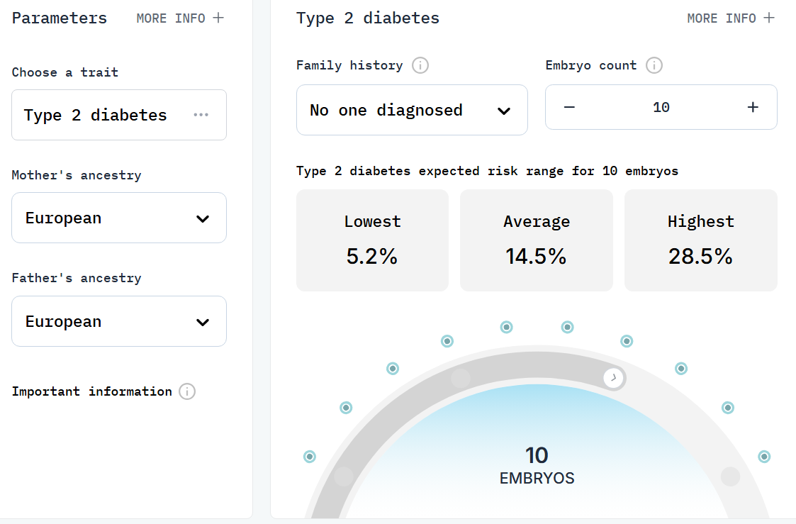
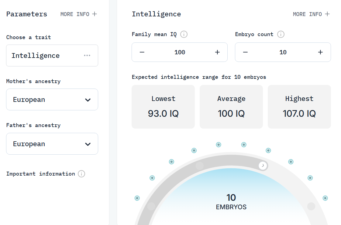
I wrote a post about embryo selection a while ago, but figured that I would write a followup after the embryo selection company Herasight was announced. They are still in stealth, but claim to be able to select embryos based on their predisposition to Alzheimer’s disease, intelligence, schizophrenia, type 2 diabetes, and several other diseases. They also display the estimated gain from embryo selection depending on the parents ancestry and the number of available embryos:
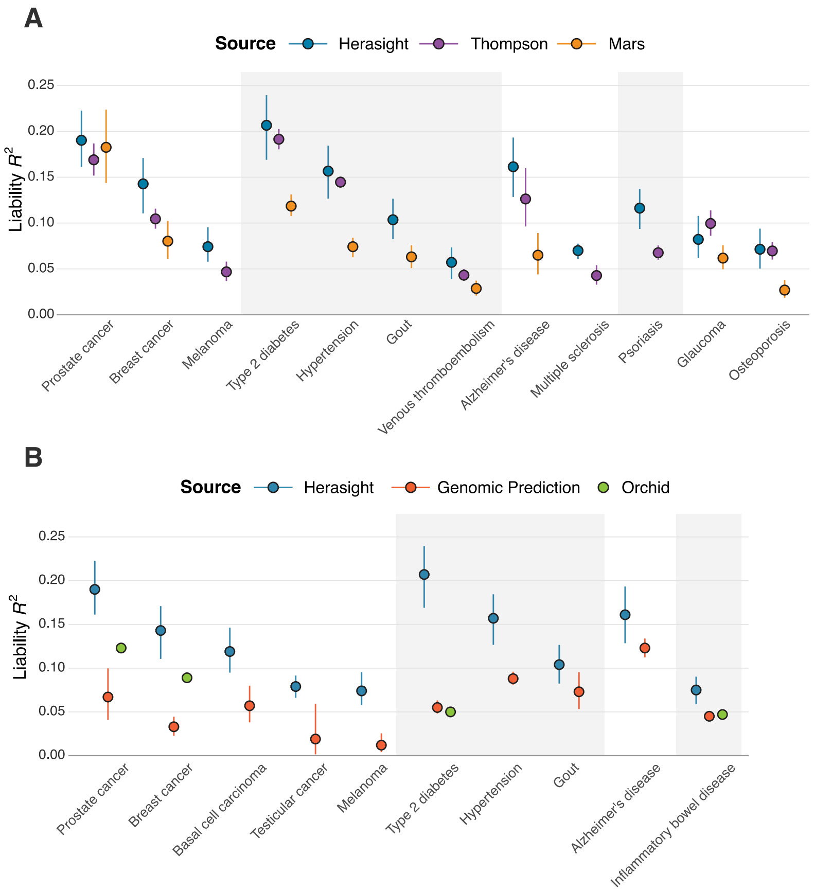
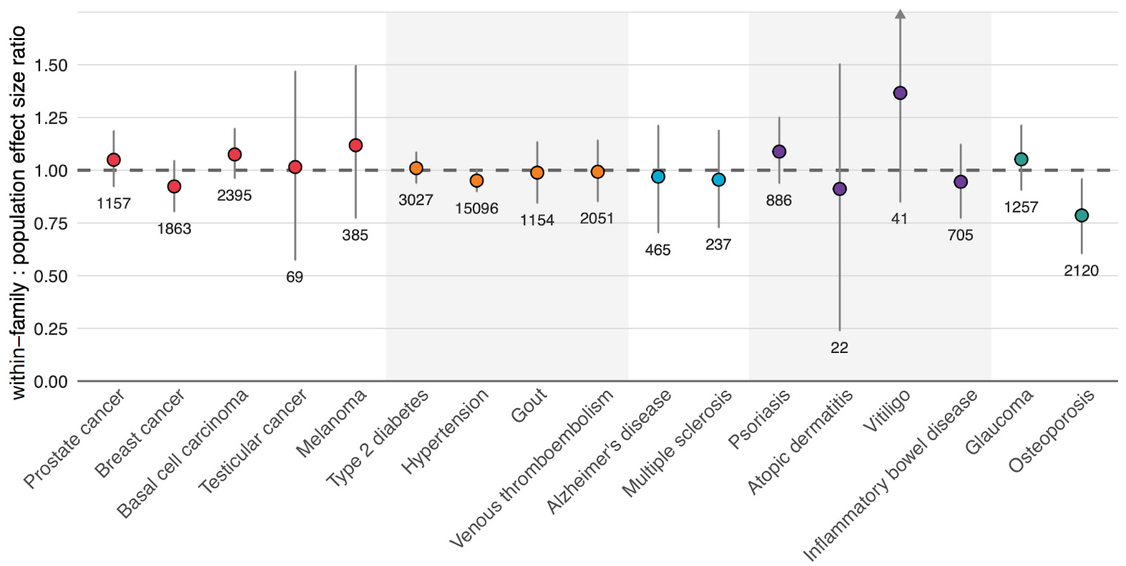
They also measured themselves up to the rest of the field, finding that their genetic prediction models for diseases were better than their competitors:
Intuitively, I’d say it is worth it: selecting for intelligence grants an estimated increase of 7 IQ points or a 2.7x reduction in a child’s risk of diabetes. Herasight do not have market prices for their services and currently charge customers based on their individual needs, butthe average cost for their customers pay is about $25,0002; customers who desire premium services can pay $50,000 for unlimited embryos for 5 years + genomic sequencing of parents/relatives.
Cost-benefit analysis
Based on available listings, I’ve estimated that the cost of IVF to be $18,0003 in the United States, the cost of genotyping the embryos is $200 per genome, and the cost of doing the embryo biopsy is about $1,500.
Other embryo selection services charge lower or similar prices4 to Herasight, but their selection methods aren’t as effective, so I’ll keep 25,000 as the current price estimate.
For the purposes of simplicity, I will assume the parents are selecting purely for intelligence (which is probably not the right thing to do). Calculating the expected gain in intelligence from embryo selection is difficult because the gain varies depending on multiple parameters, such as the number of embryos available, likelihood of mascarriage, and implantation failure.
Fortunately, Gwern has already developed a pipeline model that estimates the gain from selection:
In vitro fertilization is a sequential probabilistic process:
harvest x eggs
fertilize them and create x embryos
culture the embryos to either cleavage (2–4 days) or blastocyst (5–6 days) stage; of them, y will still be alive & not grossly abnormal
freeze the embryos
optional: embryo selection using quality and PGS
unfreeze & implant 1 embryo; if no embryos left, return to #1 or give up
if no live birth, go to #6
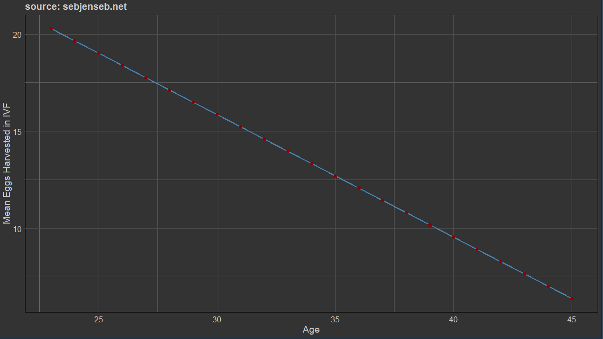
Using two studies on the mean number of eggs harvested per woman (one from America (2019), another from Singapore (2014))5, I was able to estimate the number of eggs harvested by woman per cycle:
Due to chromosomal abnormalities, some embryos cannot be fertilised and are discarded in the process; usually about 70% remain, depending on the age of the mother. After the fertilization process, the embryo is cultured in vitro to become a blastocyst; in both of the samples gwern cited in his article, about 96% of the fertilized embryos were viable for implantation. From there, the best embryo is implanted; if there is no live birth, the second best is implanted, and so on. I’ve been told that at the best clinics, the live birth success is about 70%, though the success rate in the entire US is about half that — 38%6.
There is also the issue of IVF patients being selected for fertility troubles, even multiple times over; more fertile IVF couples will exit the process with a live birth earlier, while less fertile ones will require multiple implantations or perhaps even multiple cycles. As such, the profitability estimate should be considered deflated. The use of donor eggs deals with the problem of selection in mothers, but not fathers, so the estimate of the success of fertilization should still be considered deflated as well.
If one were to personalize the 5 numbers that dictate the efficacy of embryo selection to that of a 30 year old white couple with no fertility troubles that uses Herasight (eggs harvested — 16, fertilisation rate — 72%, successful maturation rate — 96%, live birth rate — 45%, predictive validity of polygenic scores for IQ — r = .42), the expected gain in intelligence is 4.96 IQ points7.
> summary(simulateIVFs(eggMean=16, eggSD=0, polygenicScoreVariance=currentpgs, normalityP=0.72, vitrificationP=.96, liveBirth=0.45))*15
Min. 1st Qu. Median Mean 3rd Qu. Max.
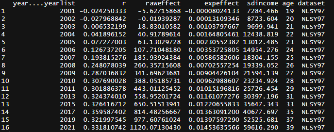
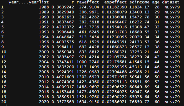
-15.334 2.837 4.956 4.970 7.126 20.404 To determine whether this cost is worth it, I took data on IQ (ASVAB) and income (self-reported) from the NLSY dataset and regressed income onto intelligence in every year, controlling for race and family background8. It turns out the 200-600$ per point estimate in Zagorsky (2007) is a massive underestimate, especially for older adults.
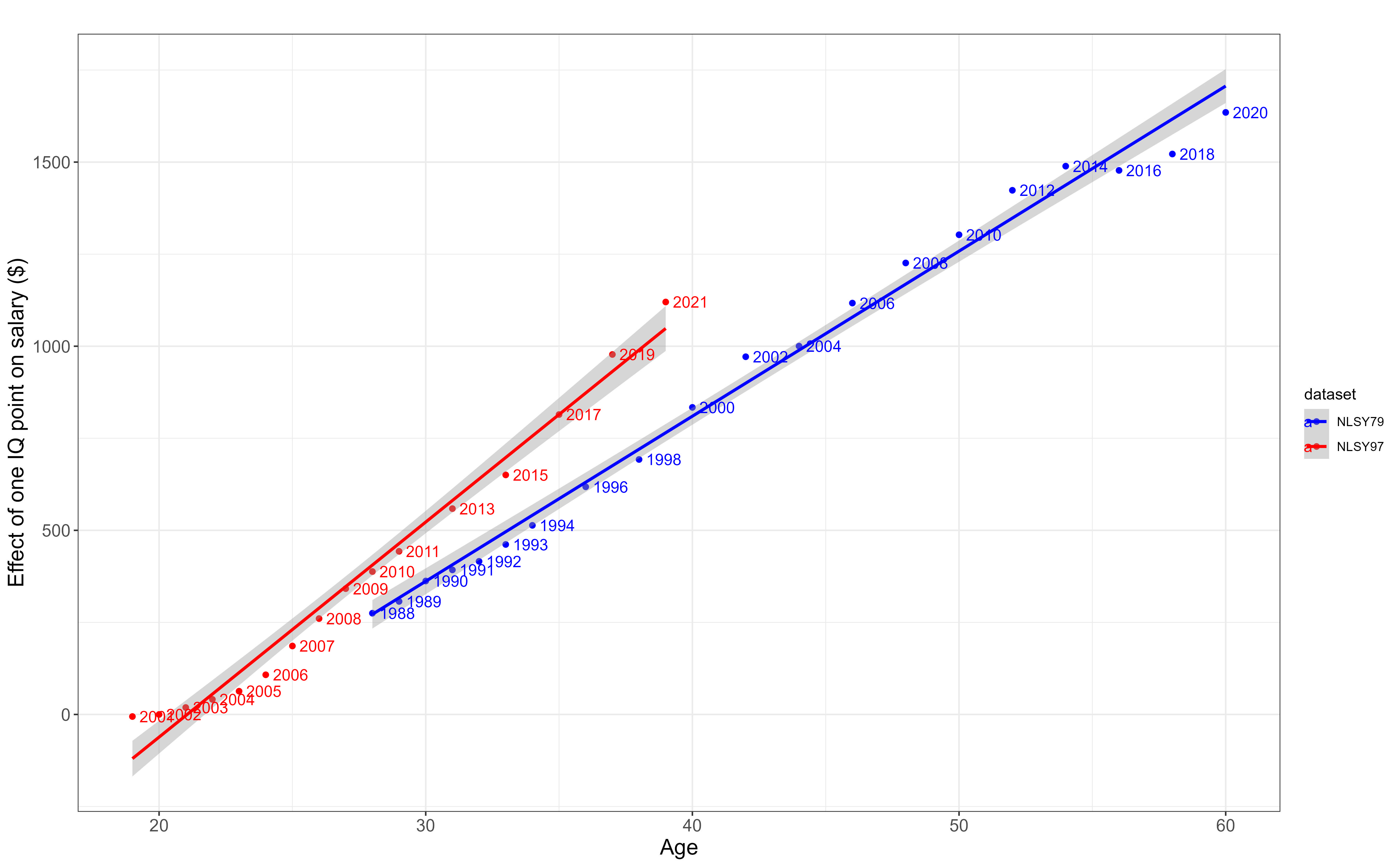
In this chart, the effect of IQ on lifelong income is the area under the curve. To quantify the uncertainty in my prediction, I measured how much the estimate varied by 4 factors: the slope (variance set to SE^2), the intercept (variance also set to SE^2), the starting age (18-22), and the ending age (65-70).
The effect of IQ on income is close to null within younger adults because most intelligent youth go to university, but it rises with age as people enter the workforce. After that, the effect of IQ on income continues to rise because the standard deviation of income rises. Older individuals still earn money after they retire through assets, but I wanted to only wanted to estimate the effects that could be statistically observed.
I found that most variants of the model estimated the effect of IQ on lifelong income to be somewhere between 40,000 and 60,0009.
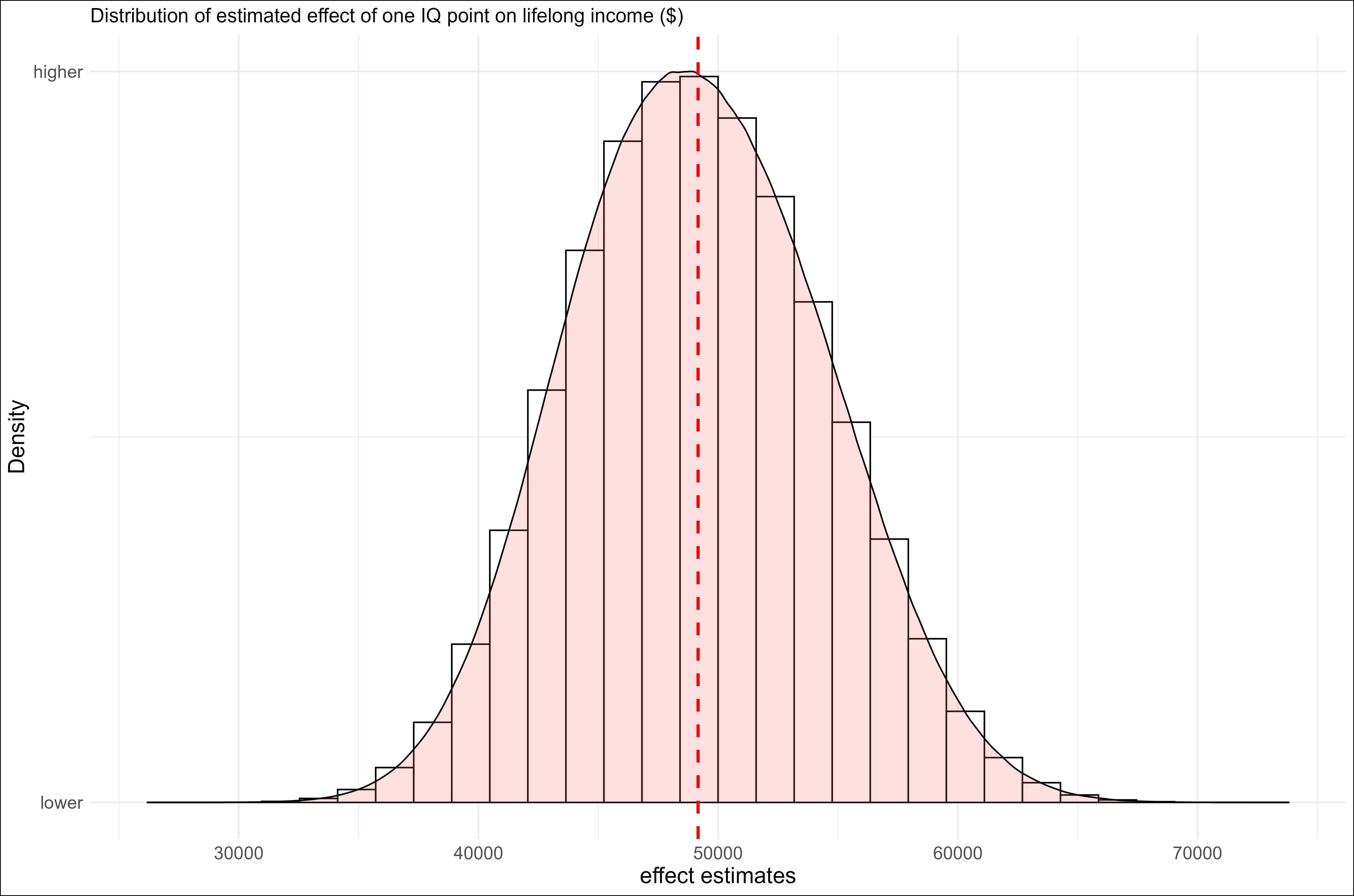
This means that those 4.96 IQ points translate to an increase in lifelong income of $240,000 for the price of $45k — IVF (~$18k) + embryo biopsy (~$2k) + embryo selection (~$25k). Even if the absolute minimum estimate of IQ’s effect on lifelong income were used ($27,000), it would still be worth it. So yes, it is profitable from a financial perspective.
Is it actually worth it?
This analysis is devoid of logic. People pay emotional and temporal costs when using IVF beyond money, and said money could also be used on other opportunities such as stocks or real estate. Intelligence also has more value beyond the income that it can provide an individual and embryo selection can be used to select for traits beyond intelligence.
In 1985, the S&P 500 was listed at $191 while in 2025 it is listed at 6,600; one could argue then that embryo selection is not worth it from the perspective of opportunity costs, though this is only true if one believes that stocks will constantly go up this century (I don’t). Forgive my ageism, but I also question whether having one million dollars as an old retiree is more valuable than having better children.
Some may see embryo selection as a status symbol which signals to others that you are aware of and willing to use avant garde esoteric scientific techniques to benefit your children. Even if it were the case that embryo selection gave people status (it’s a weird rich people thing), I would not advocate for doing it for that reason. Optimizing for status at the cost of other values is slavish and leads to one internalizing the values of others rather than those of the self.
I also considered calculating the profitability of embryo selection depending on characteristics like the age and race of the mother, but I thought it went without saying that the value of embryo selection itself depends strongly on the couple. The impact on race on the efficacy of embryo selection is rather small in most races except Africans: European couples selecting 1 embryo of 10 for intelligence should expect a gain of 7 IQ points; Hispanics 6.3, Middle Easterners 6.1, East Asians 5.4, South Asians 6.3, and Africans 4.
I should also mentiont that the costs of doing embryo selection should decrease in the future as the space gets more competitive and technology advances, not to mention the accuracy of the genetic prediction models. As such, the monetary analysis should become more and more tilted towards the side of doing embryo selection over time. I also may or may not have heard about a new way of genetically sequencing embryos…

Ethics of embryo selection
Once a live birth in IVF occurs, parents can choose to keep their embryos fertilised for the purposes of future births, donate them, or dispose of them. One could argue that the disposal of embryos constitutes murder as the embryos are living beings. From a consequential perspective, if a couple wants to have children, they can do so naturally or using IVF. Both of these decisions result in identical increments in total life: 10-9 and 1 are the same number.
Another concern people have about embryo selection is that it could lead to negative social or political outcomes; people might be discriminated against for being naturally conceived and embryo selection could lead to increased social inequality. With regards to discrimination, I think it is unlikely that genetically enhanced children would be advantaged in employment or university admissions; genetic discrimination is already illegal in the United States in health and employment and even if it wasn’t, I don’t think that companies would be super invested into hiring employees who were embryo selected.
Even if genetically-based discrimination were to become common, I don’t see how it’s any worse than discriminating based on education. Both correlate with productivity, but the value of education is zero sum (involves investing resources and time into signalling you are more productive than other people) while genetic enhancement gives people different genes. I also think it’s unlikely that embryo selection will ever be popular in the near future; as of now it takes a lot of money, energy, and time to use it.
People also have qualms about adverse selection occurring, for example, people selecting for increasingly tall sons would only result in the goalposts for being “tall” or “short” being shift. Personally, I think it would be cool if humans became 7’ tall giants, though it would be bad if it got too out of hand…
Some are concerned that monomaniacally selecting children for IQ could lead to a society filled to the brim with nerds or losers. Empirically, highly intelligent people also tend to be slightly taller, more attractive10, and popular in school. The nerd as a type definitely exists but selecting people for intelligence will not make them more “nerdy”, per say.
Alternatively, one could be concerned about selection for high levels of intelligence could result in there being more dysfunctional geniuses because high levels of intelligence cause maladjustment. This is not borne out in data: intelligent (>2 SD) people are at lower risks for most mental and physiological disorders with the exception of myopia and autoimmune disorders.

The only obvious downside of selecting children for intelligence is autism and the risk is not that relevant — autism and IQ genetically correlate at about .2 - .3, so increasing a child’s IQ by 6 points would lead to them being only 0.1 SD more autistic. If we got to the point that embryo selection or a related procedure were to be able to increase IQ by 45 points, then it would also make people 0.75 SD more autistic. Which is a pretty large effect, though it seems like a small price to pay for an IQ of… 145.
The idea that embryo selection is “racist” or “eugenics” is a smear — is wanting to date tall men “eugenics”? Are incest-avoidant taboos eugenic? What is attempted here is a conflation between the genocidal and forceful eugenics of the 20th century and a scientific process that allows parents to select between different embryos to implant.
Does this actually work as advertised?
Yes.
The polygenic scores that are used to select the embryos are generated by observing which genetic variants predict traits in the general population. Although everything is genetic (at least partially), the models themselves make no assumptions about the heritability of traits within the general population. All they do is assume that the genetic variants that are correlated with traits reflect causal associations.
Which isn’t much of a strech. Say, if you had a population that was 50% Chinese and 50% English, people with straighter hair would be more likely to be short, so naive genetic prediction models would assume that the genes that make people short also give them straight hair. Fortunately, these studies correct for this by calculating the first principal components (usually a large number, like 10 or 20) of the genetic data, which maps onto whatever racial or geographic variation that exists in the studied population; some simply exclude individuals of non-European ancestry. See the most recent height GWAS, for example:
Samples used for prediction and estimation of variance explained We quantified the accuracy of a PGS based on GWS SNPs as well as the variance explained by SNPs within GWS loci, in eight different datasets independent of our discovery GWAS meta-analyses. These datasets include two samples of EUR from the UKB (n = 14,587) and the Lifelines study (n = 14,058), two samples of AFR from the UKB (n = 6,911) and the PAGE study (n = 8,238), two samples of EAS (n = 2,246) from the UKB and the China Kadoorie Biobank (CKB; n = 47,693), one sample of SAS from the UKB (n = 9,257) and one sample of HIS from the PAGE study (n = 4,939). Analyses were adjusted for age, sex, 20 genotypic principal components
Some have noted that the predictive validity of polygenic scores within families is weaker than the predicitve validity between families. This is getting extremely technical, but bear with me: this can happen for two reasons. One is that the polygenic scores are picking up on environmental variance that causes trait values (like parenting or social class) or that assortative mating leads to parental genotypes being a proxy for child genotypes because polygenic scores pick up on noncausal variants that are correlated with causal variants through linkeage disequilibrium (non-random associations between genes in different locations; this is extremely hard to understand without relevant background knowledge).
If it is the former, then embryo selection will not work as advertised, as part of the reason why these genes predict trait values is because they are correlated with environments that the selected embryos will not have. If it’s just assortative mating, then the lower prediction accuracy within families is an artefact and therefore not relevant to prediction.
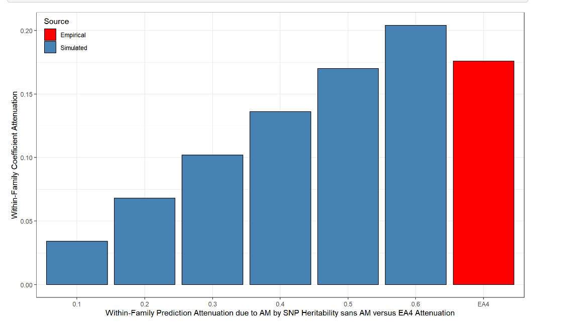
Somebody else has already tried assessing the extent to which within-family attenuation can be inferred to be due to assortment (based on the empirical correlation in IQ between family members) and the baseline heritability of intelligence. He estimated all of the attenuation to be due to assortment.
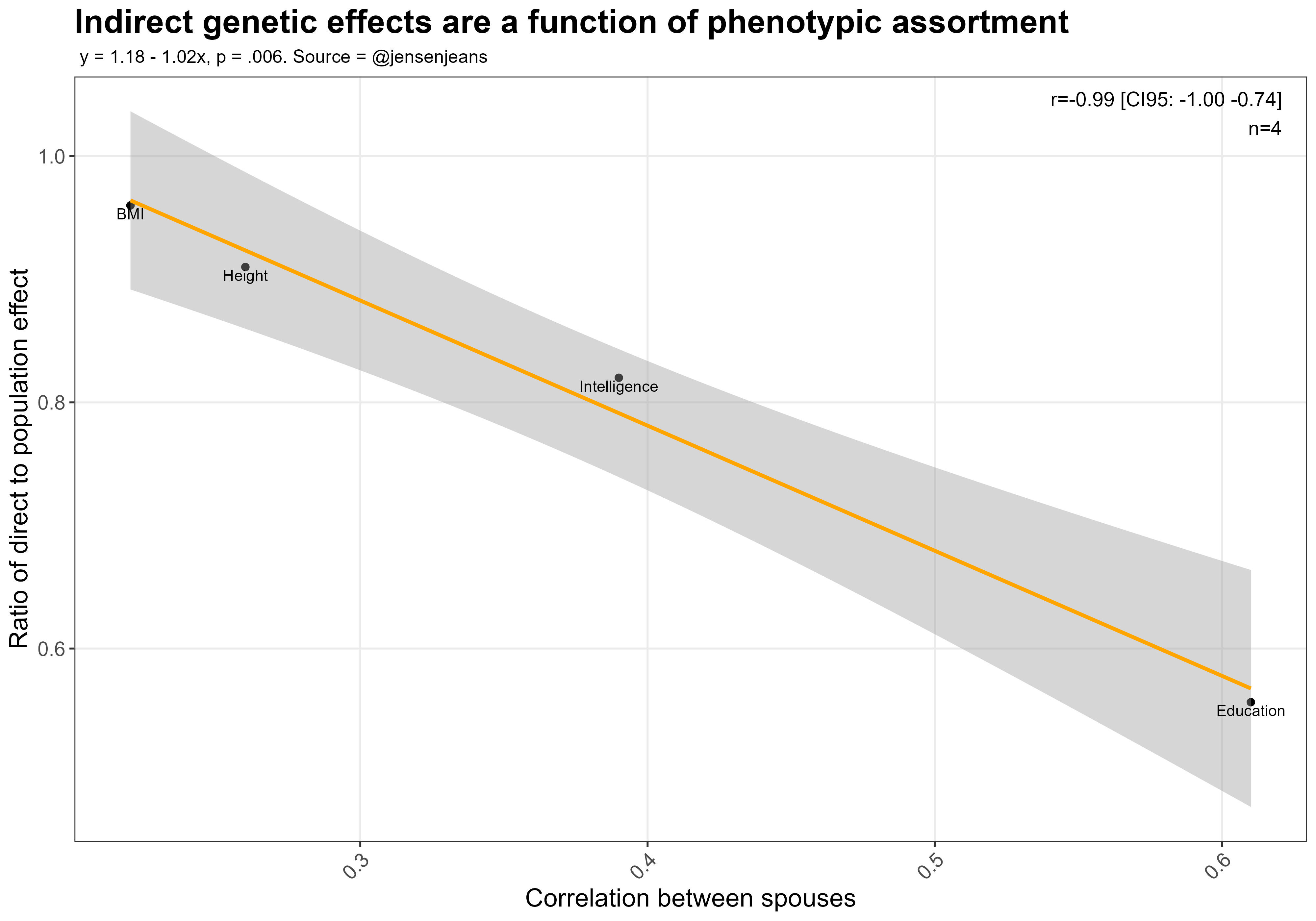
I also tried testing this by examining whether traits with greater within-family attenuation were more strongly assorted for. Based on the limited evidence available, the indirect genetic effects seem to be a function of phenotypic assortment (and heritabilities, presumably):
I should also mention that Herasight did not find diminished predictive accuracy within families:
Wrap up
Yes. It works. Do it if it aligns with your values and circumstances.
Currently, I would recommend selecting children for intelligence and against type 2 diabetes; both phenotypes are about equally valuable and dying of prostate cancer at the age of 70 isn’t very different from dying from a stroke at the age of 80, but living life as a diabetic and non-diabetic is very different.
Numbers which estimate an individual’s genetic liability to a trait. Usually derived from GWAS (genome wide association study), which are studies that measure the association between genes and a given trait.
source: personal correspondence.
Gwern estimates the cost of IVF to be somewhere between 8,000 and 20,000 USD. This appears to have been accurate at the time, though the cost of IVF appears to have increased in recent years, with sources reporting figures in these ranges: 15,000-30,000, 10,000, 14,000-20,000, 20,000, and 15,000 - 20,000. The absolute interval for the cost is $10,000 - $30,000, and the mean is $18000 (a friend of mine told me that IVF costs 5k USD in Czechia, and that splitkits can be used to reduce the cost of sequencing the embryos).
Nebula is currently selling whole genome kits for $195, which would be the cost of selecting a single embryo for genes.
There is also an additional cost that arises from choosing to do polygenic testing itself. Gwern finds that, based on public cost data, the price of genetic testing is about $4,000, but that most of this cost is due to the embryo freezing and genetic screening; the former must be done regardless of whether embryo selection is carried out and the cost of the latter can be estimated using kits. The embryo biopsy, which is the necessary process to test embryos genetically costs only about 1,000 - 2,000 USD or so.
See Scott Alexander’s review:
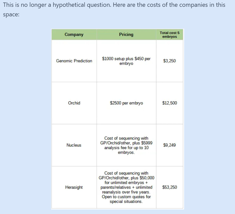
Table:
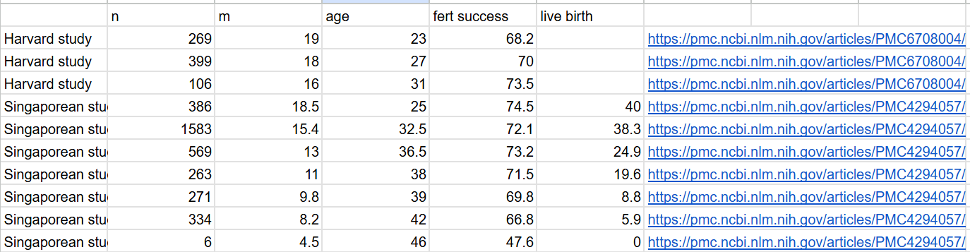
I ran a linear regression of mean eggs ~ age to estimate the mean number of eggs harvested, and then mutliplied that by the likelihood of fertilisation success to get the total number of eggs available. The Singapore study uses patients who are seeking IVF, the Harvard study looks at women who are using donor eggs.

Code. Also, increasing the egg SD above 0 only increased the expected gain, from what I saw.
simulateIVF <- function (eggMean, eggSD, polygenicScoreVariance, normalityP=0.5, vitrificationP, liveBirth) {
  eggsExtracted <- max(0, round(rnorm(n=1, mean=eggMean, sd=eggSD)))
  normal        <- rbinom(1, eggsExtracted, prob=normalityP)
  scores        <- rnorm(n=normal, mean=0, sd=sqrt(polygenicScoreVariance*0.5))
  survived      <- Filter(function(x){rbinom(1, 1, prob=vitrificationP)}, scores)
  selection <- sort(survived, decreasing=TRUE)
  if (length(selection)>0) {
    for (embryo in 1:length(selection)) {
      if (rbinom(1, 1, prob=liveBirth) == 1) {
        live <- selection[embryo]
        return(live)
      }
    }
  }
}
simulateIVFs <- function(eggMean, eggSD, polygenicScoreVariance, normalityP, vitrificationP, liveBirth, iters=100000) {
  return(unlist(replicate(iters, simulateIVF(eggMean, eggSD, polygenicScoreVariance, normalityP, vitrificationP, liveBirth))));
}Methodology:
Parental SES in the NLSY79 dataset was calculated using the education and occupation of the parents, while in the NLSY97 dataset it was calculated using assets, income, mother’s education, and father’s education. Race was measured using self-identification and income was measured using self-reports. IQ was measured using the first principal component of the ASVAB datasets.
Tables for the charts:
Distribution:

I don’t think selecting children for intelligence will lead to measurable gains in either of these traits.
Loved the article, just a point on the finance side: as others noted, you should apply a discount rate. If I pay 10,000 USD today and receive 10,000 USD back in 20 years, I did not breakeven, I lost money. This has to be accounted for.
Great article, but one minor nitpick:
“as the majority of the people using this technology will likely be White.”
This would be true initially, but perhaps not eventually, and certainly not worldwide long-term.