What kind of people are really into anime?

a study of the OKCupid (2014-2015) dataset

May 23, 2025

TL;DR: people who claim to be really into anime are more likely to be men, childless, poor, bicurious, nonwhite, racist, unathletic, bullied in high school, into Asians, kinky, unconscientious, and eccentric.

Intelligence and height were uncorrelated with liking anime.

Full list of predictors of liking anime:

Being male.
Being bisexual (regardless of sex).
Having a sexual ecounter with the same sex or wanting one.
Not being gay (within men).
Not having children.
Being young.
Having poor hygeine habits.
Being either skinny or fat.
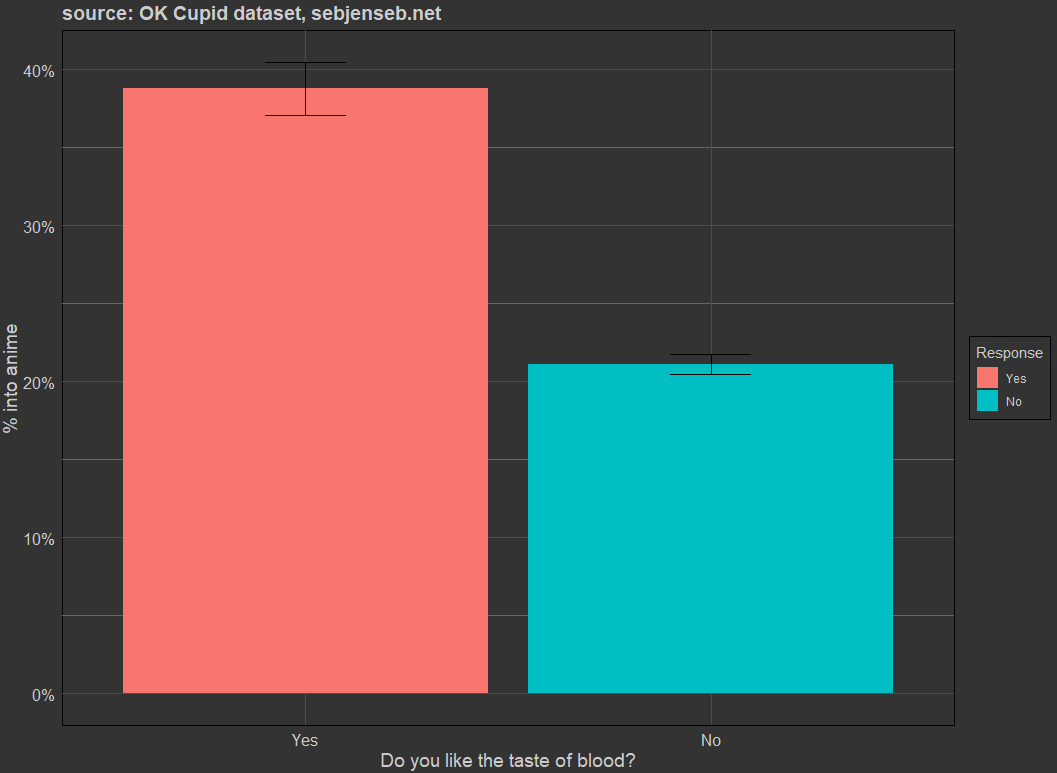
Liking the taste of blood (surprisingly large effect — ~21% for no and ~39% for yes).
Low income (people into anime make 10,000$ less, controlling for race/sex/sexuality/age).
No association between field of employment and liking anime survives controls for sex, race, age, and income.
Being a college dropout or student.
Taking drugs.
Being a Buddhist, Muslim, or Atheist; not a Christian.
Being Asian, Hispanic, or Black; not White or Indian.
(if black or asian) not viewing race as a core part of your identity.
(if white) viewing race as a core part of your identity.
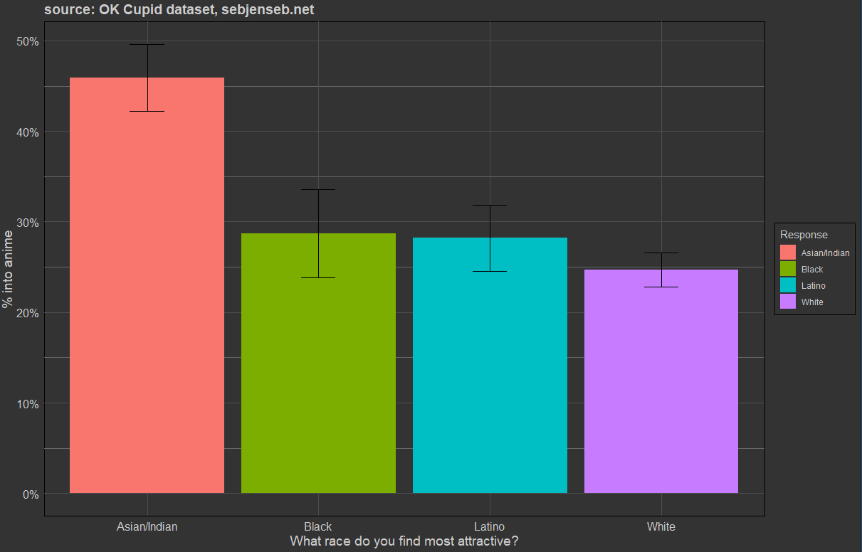
Claiming to find Asians attractive (regardless of race or sex).
Finding foreign accents sexy.
Being comfortable with racist jokes (effect is specific to men).
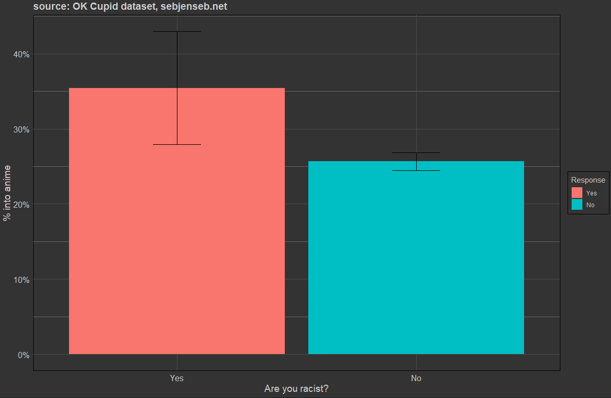
Claiming to be racist.
Living in Turkey, the Philippines, Sweden, Australia, Peru, or Trinidad.
Not living in DC, Germany, Illinois, Indiana, Maryland, the Netherlands, New York, Ontario, Oklahoma, or Pennsylvania.
Not having left one’s country of origin.
Non-conservative political beliefs.
Being willing to date a shorter partner (if female). Some of this is due to convariance with a preference for Asians.
Having rape fantasies (regardless of sex)
Having LGBT friends.
Not thinking that bisexual people are more likely to be unfaithful.
Using the word ‘gay’ as a prejorative.
Not claiming to have been a “cool kid” in high school.
Claiming to have been picked on a lot in school.
Being less close to your family.
Claiming to be unticklish.
Reporting lower levels of attractiveness relative to other individuals
Being into bondage.
Believing in ghosts.
Wearing a lot of black.
Disliking chivalry
Supporting restrictions on the number of children that a family can have.
Supporting nuclear energy.
Preferring to send rather than receive messages (?).
Thinking that it should not be a jailable offense to have sex with a 16 year old as a 25+ year old.
Viewing laziness as a cause of homelessness.
Thinking there should be more or less humans on the planet.
Thinking people of colour can’t be racist.
Thinking the world would be a better place if low IQ people couldn’t reproduce
Thinking seuxal assault accusations at the workplace made by women are false.
Ambivalent attitudes towards feminism (if female).
Ambivalent or positive attitudes towards feminism (if male).
Being willing to take off one’s shirt in the nightclub.
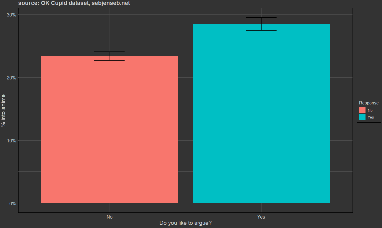
Enjoying arguing.
Claiming to be unhappy with one’s life.
Claiming to be less ambitious (d = -.25), more independent (d = .12), more romantic (d = .1) more kinky (d = .32), less optimistic (d = -.24), more into literature (d = .15), less into politics (d = -.17), having worse manners (d = -.25), more sloppy (d = .13), more indie (d = .34), more introverted (d = .13), more trusting (d = .25), more thrifty (d = .38), less organized (d = -.16), experienced in sex (d = .1), artsy (d = .21), spontaneous (d = .18), giving (d = .12), less experienced in love (d = -.18), less conventionally moral (d = -.15), less kind (d = -.14), less friendly to strangers (d = -.13), less old-fashioned (d = -.28), less energetic (d = -.21), less into exercise (d = -.23), more into math (d = .16), geeky (d = 1.21), and adventurous (d = .18).

Things that were uncorrelated with liking anime:

Nationality and location, in most cases.
Height
Believing in the existence of a correlation between race and intelligence.
Being Jewish.
Blushing easily.
IQ.
Claiming to be confident, being laid back, being into drugs, being progressive, being dominant, being submissive, arrogant, cool, have a high sex drive, honest, into science, experienced in life, greedy, capitalistic, aggressive, extraverted (surely this is wrong?), competitive, driven by love, spirited, passionate
Disliking promiscuous people.
Being into abstract art.
Being disgusted by extremely obese people

The statistics in this post are based on the OK Cupid dataset, a scraped sample of 68,371 individuals who used the OK Cupid website. Some participants answered whether they were “really into Japanese Animation (anime) movies” — 20,000 people answered and 25% said yes.

Given the large sample size, I didn’t bother engaging in significance testing, as even the smallest effects pass significance. For example, people who had LGBT friends were really into anime 24% of the time, while those who did not were really into anime 21% of the time. This difference passed statistical significance easily:

> okcdataset %>% group_by(q7085) %>% summarise(into_anime = mean(anime, na.rm=T), sum(!is.na(anime)))
# A tibble: 3 × 3
  q7085 into_anime `sum(!is.na(anime))`
  <chr>      <dbl>                <int>
1 No        0.2136                 2154
2 Yes       0.2437                13465
3 NA        0.2824                 8173


table_data <- table(q7085 = okcdataset$q7085, anime = okcdataset$anime)
> chisq.test(table_data)

	Pearson's Chi-squared test with Yates' continuity correction

data:  table_data
X-squared = 9.1232, df = 1, p-value = 0.002524

I looked through the list of questions the participants were asked, tallied the ones that looked interesting, and ran the R code.

I charted the best results:

There was no difference in measured intelligence; I copied the method Kirkegaard uses to calculate IQ, and subset the sample to those who answered at least 5 questions:

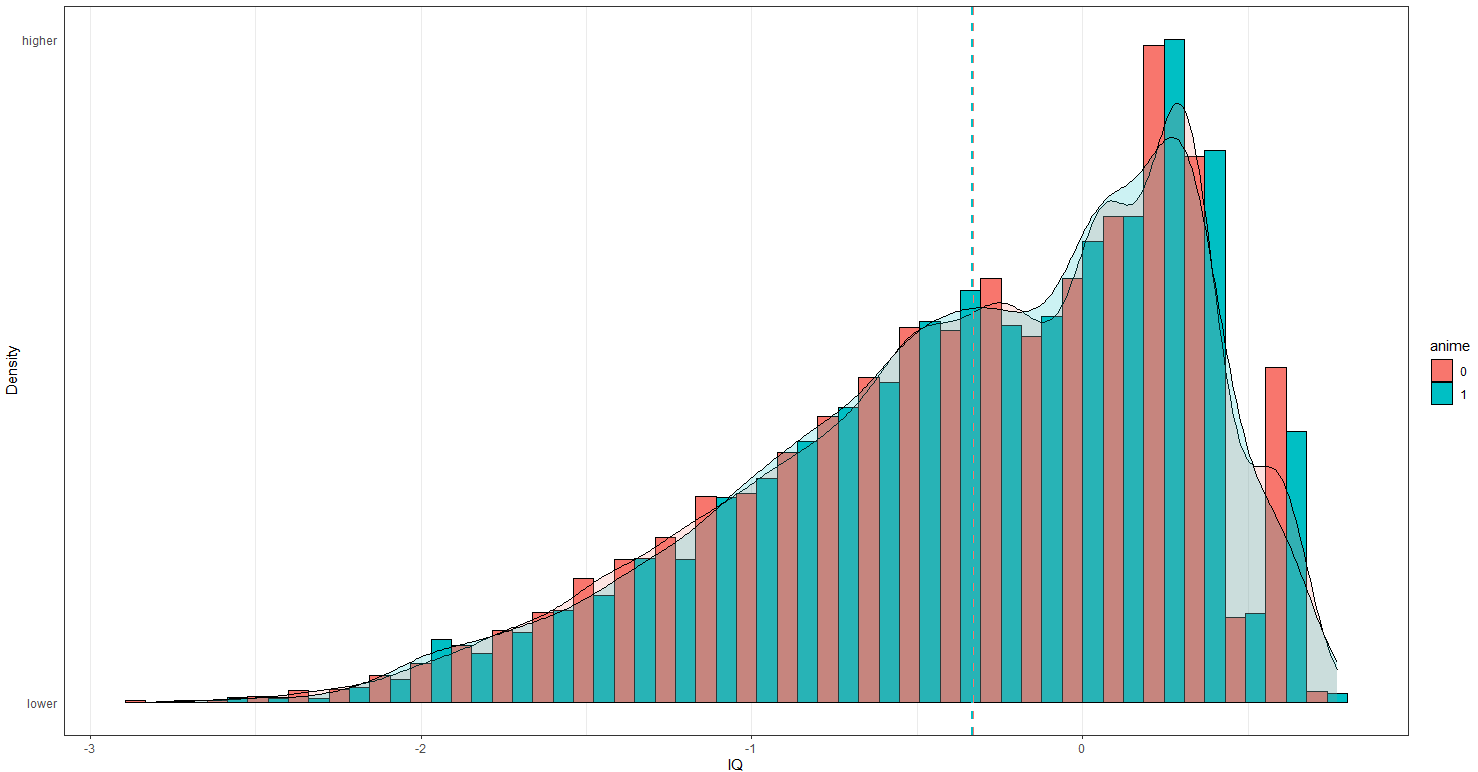
The association did become positive after controlling for race/sex/sexuality/income:

> summary(lr)

Call:
lm(formula = anime ~ IQ + race + sex + sexuality + numincome, 
    data = d)

Residuals:
    Min      1Q  Median      3Q     Max 
-0.7438 -0.2992 -0.2395  0.5426  1.5853 

Coefficients:
                              Estimate    Std. Error t value             Pr(>|t|)    
(Intercept)               0.1647436287  0.0143720806  11.463 < 0.0000000000000002 ***
IQ                        0.0233550072  0.0085601642   2.728              0.00638 ** 
raceAsian                 0.2636851982  0.0418578199   6.300   0.0000000003187740 ***
raceBlack                 0.1818156689  0.0309390413   5.877   0.0000000044034711 ***
raceHispanic / Latin      0.1393756141  0.0296596412   4.699   0.0000026680088361 ***
raceIndian               -0.0666111519  0.0785596379  -0.848              0.39652    
raceMiddle Eastern        0.0806213268  0.1260831090   0.639              0.52257    
raceOther                 0.0644259638  0.0387806243   1.661              0.09670 .  
racePacific Islander      0.4396059473  0.1380291450   3.185              0.00146 ** 
raceSelected over 1 race  0.1395538637  0.0185229402   7.534   0.0000000000000561 ***
sexMale                   0.1830984905  0.0140346037  13.046 < 0.0000000000000002 ***
sexualityBisexual         0.1663696674  0.0228315753   7.287   0.0000000000003564 ***
sexualityGay             -0.0045087442  0.0246157412  -0.183              0.85467    
sexualityOther            0.0630129728  0.0842310494   0.748              0.45443    
numincome                -0.0000012188  0.0000001102 -11.063 < 0.0000000000000002 ***
---
Signif. codes:  0 ‘***’ 0.001 ‘**’ 0.01 ‘*’ 0.05 ‘.’ 0.1 ‘ ’ 1

Residual standard error: 0.4358 on 6271 degrees of freedom
  (22433 observations deleted due to missingness)
Multiple R-squared:  0.06421,	Adjusted R-squared:  0.06212 
F-statistic: 30.73 on 14 and 6271 DF,  p-value: < 0.00000000000000022

…Which is an artefact of controlling for income, which should not be done, as personal income does not cause IQ. It just means that the non-income variance in IQ is positively correlated with liking anime.

R code:

#Sexuality coding:
okcdataset$sexuality <- okcdataset$d_orientation
okcdataset$sexuality[okcdataset$sexuality=="Pansexual"] <- "Bisexual"
okcdataset$sexuality[okcdataset$sexuality=="Straight, Gay"] <- "Bisexual"
okcdataset$sexuality[okcdataset$sexuality=="Heteroflexible"] <- "Bisexual"
okcdataset$sexuality[okcdataset$sexuality=="Homoflexible"] <- "Bisexual"
okcdataset$sexuality[okcdataset$sexuality=="Lesbian"] <- "Gay"
okcdataset$sexuality[okcdataset$sexuality=="Bisexual, Pansexual"] <- "Bisexual"
okcdataset$sexuality[okcdataset$sexuality=="Straight, Bisexual"] <- "Bisexual"
okcdataset$sexuality[okcdataset$sexuality=="Straight, Bisexual, Heteroflexible"] <- "Bisexual"
okcdataset$sexuality[okcdataset$sexuality=="Straight, Pansexual"] <- "Bisexual"
okcdataset$sexuality[okcdataset$sexuality=="Heteroflexible, Bisexual"] <- "Bisexual"
okcdataset$sexuality[okcdataset$sexuality=="Pansexual, Bisexual"] <- "Bisexual"
okcdataset$sexuality[okcdataset$sexuality=="Homoflexible, Heteroflexible, Pansexual, Bisexual"] <- "Bisexual"
okcdataset$sexuality[!(okcdataset$sexuality=="Bisexual" | okcdataset$sexuality=="Straight" | okcdataset$sexuality=="Gay" | is.na(okcdataset$sexuality))] <- "Other"

#Race coding:
okcdataset$race <- okcdataset$d_ethnicity
okcdataset$race[!(okcdataset$d_ethnicity=='Asian' | okcdataset$d_ethnicity=='Black' | okcdataset$d_ethnicity=='Indian' | okcdataset$d_ethnicity=='White' | okcdataset$d_ethnicity=='Hispanic / Latin' | okcdataset$d_ethnicity=='White' | okcdataset$d_ethnicity=='Middle Eastern' | okcdataset$d_ethnicity=='Pacific Islander' | okcdataset$d_ethnicity=='Other' | is.na(okcdataset$d_ethnicity))] <- 'Selected over 1 race'






Call:
lm(formula = anime ~ IQ + race + sex + sexuality, data = d)

Residuals:
    Min      1Q  Median      3Q     Max 
-0.6992 -0.2494 -0.2453  0.4451  0.9365 

Coefficients:
                          Estimate Std. Error t value             Pr(>|t|)    
(Intercept)               0.102364   0.006663  15.362 < 0.0000000000000002 ***
IQ                        0.002616   0.004801   0.545              0.58582    
raceAsian                 0.202613   0.015975  12.683 < 0.0000000000000002 ***
raceBlack                 0.164589   0.016303  10.096 < 0.0000000000000002 ***
raceHispanic / Latin      0.125546   0.015795   7.949  0.00000000000000199 ***
raceIndian               -0.069057   0.034661  -1.992              0.04635 *  
raceMiddle Eastern        0.098434   0.052654   1.869              0.06158 .  
raceOther                 0.093367   0.019344   4.827  0.00000139858133607 ***
racePacific Islander      0.271782   0.069745   3.897  0.00009778746816569 ***
raceSelected over 1 race  0.122779   0.010170  12.072 < 0.0000000000000002 ***
sexMale                   0.146296   0.006996  20.911 < 0.0000000000000002 ***
sexualityBisexual         0.181169   0.012360  14.657 < 0.0000000000000002 ***
sexualityGay             -0.034171   0.012304  -2.777              0.00549 ** 
sexualityOther            0.062387   0.038580   1.617              0.10587    
---
Signif. codes:  0 ‘***’ 0.001 ‘**’ 0.01 ‘*’ 0.05 ‘.’ 0.1 ‘ ’ 1

Residual standard error: 0.4235 on 19425 degrees of freedom
  (9280 observations deleted due to missingness)
Multiple R-squared:  0.046,	Adjusted R-squared:  0.04536 
F-statistic: 72.05 on 13 and 19425 DF,  p-value: < 0.00000000000000022

> okcdataset %>% group_by(gender) %>% summarise(into_anime = mean(anime, na.rm=T), sum(!is.na(anime)))
# A tibble: 4 × 3
  gender into_anime `sum(!is.na(anime))`
  <chr>       <dbl>                <int>
1 Man        0.2862                15643
2 Other      0.3417                  120
3 Woman      0.1697                 7296
4 NA         0.4011                  733

> okcdataset %>% group_by(sexuality, gender) %>% summarise(anime_like = mean(anime, na.rm=T), sum(!is.na(anime)))
`summarise()` has grouped output by 'sexuality'. You can override using the `.groups` argument.
# A tibble: 13 × 4
# Groups:   sexuality [5]
   sexuality gender anime_like `sum(!is.na(anime))`
   <chr>     <chr>       <dbl>                <int>
 1 Bisexual  Man        0.4556                  496
 2 Bisexual  Other      0.55                     20
 3 Bisexual  Woman      0.3344                 1259
 4 Gay       Man        0.2437                 1149
 5 Gay       Other      0.125                     8
 6 Gay       Woman      0.1841                  315
 7 Other     Man        0.3871                   62
 8 Other     Other      0.3077                   78
 9 Other     Woman      0.2093                   86
10 Straight  Man        0.2832                13936
11 Straight  Other      0.3571                   14
12 Straight  Woman      0.1315                 5636
13 NA        NA         0.4011                  733

> okcdataset %>% filter(d_ethnicity=='Asian' | d_ethnicity=='Black' | d_ethnicity=='Indian' | d_ethnicity=='White' | d_ethnicity=='Hispanic / Latin' | d_ethnicity=='Middle Eastern' | d_ethnicity=='Pacific Islander' | d_ethnicity=='Other') %>% group_by(d_ethnicity) %>% summarise(into_anime = mean(anime, na.rm=T), sum(!is.na(anime)))
# A tibble: 8 × 3
  d_ethnicity      into_anime `sum(!is.na(anime))`
  <chr>                 <dbl>                <int>
1 Asian                0.3983                  836
2 Black                0.3766                  802
3 Hispanic / Latin     0.3481                  856
4 Indian               0.1698                  159
5 Middle Eastern       0.3014                   73
6 Other                0.3207                  555
7 Pacific Islander     0.4524                   42
8 White                0.2171                16203


q12	Divide your age by 2.  Have you had sex with at least that many people?

> okcdataset %>% group_by(q12) %>% summarise(into_anime = mean(anime, na.rm=T), sum(!is.na(anime)))
# A tibble: 3 × 3
  q12   into_anime `sum(!is.na(anime))`
  <chr>      <dbl>                <int>
1 No        0.2755                 9428
2 Yes       0.2347                 5671
3 NA        0.2441                 8693


q13	Is a girl who's slept with 100 guys a bad person?
q14	Is a guy who's slept with 100 girls a bad person?

> okcdataset %>% group_by(q13) %>% summarise(into_anime = mean(anime, na.rm=T), sum(!is.na(anime)))
# A tibble: 3 × 3
  q13   into_anime `sum(!is.na(anime))`
  <chr>      <dbl>                <int>
1 No        0.2557                18274
2 Yes       0.2367                 2505
3 NA        0.2605                 3013

> okcdataset %>% group_by(q14) %>% summarise(into_anime = mean(anime, na.rm=T), sum(!is.na(anime)))
# A tibble: 3 × 3
  q14   into_anime `sum(!is.na(anime))`
  <chr>      <dbl>                <int>
1 No        0.2530                17598
2 Yes       0.2531                 2940
3 NA        0.2624                 3254

q51	Do you think really abstract art—like just splattered paint—can be truly brilliant?

> okcdataset %>% group_by(q51) %>% summarise(into_anime = mean(anime, na.rm=T), sum(!is.na(anime)))
# A tibble: 3 × 3
  q51   into_anime `sum(!is.na(anime))`
  <chr>      <dbl>                <int>
1 No        0.2470                 7057
2 Yes       0.2406                 8939
3 NA        0.2766                 7796

q65	Do you have a problem with racist jokes?

> okcdataset %>% group_by(q65) %>% summarise(into_anime = mean(anime, na.rm=T), sum(!is.na(anime)))
# A tibble: 3 × 3
  q65   into_anime `sum(!is.na(anime))`
  <chr>      <dbl>                <int>
1 No        0.2926                10814
2 Yes       0.2185                10273
3 NA        0.2370                 2705

q57	Do you like to argue?


> okcdataset %>% group_by(q57) %>% summarise(into_anime = mean(anime, na.rm=T), sum(!is.na(anime)))
# A tibble: 3 × 3
  q57   into_anime `sum(!is.na(anime))`
  <chr>      <dbl>                <int>
1 No        0.2338                14061
2 Yes       0.2850                 7298
3 NA        0.2803                 2433

q18781	Do you agree with the statement 'everyone's a little racist'?

> okcdataset %>% group_by(q18781) %>% summarise(into_anime = mean(anime, na.rm=T), sum(!is.na(anime)))
# A tibble: 3 × 3
  q18781 into_anime `sum(!is.na(anime))`
  <chr>       <dbl>                <int>
1 No         0.2390                 2188
2 Yes        0.2849                 2738
3 NA         0.2516                18866

q163	If a poor 20 year-old woman marries a wealthy 40 year-old man, do you assume it's for the money?


> okcdataset %>% group_by(q163) %>% summarise(into_anime = mean(anime, na.rm=T), sum(!is.na(anime)))
# A tibble: 3 × 3
  q163  into_anime `sum(!is.na(anime))`
  <chr>      <dbl>                <int>
1 No        0.2622                 6118
2 Yes       0.2170                 5866
3 NA        0.2687                11808

q177	Which better explains why most homeless people are homeless?


> okcdataset %>% group_by(q177) %>% summarise(into_anime = mean(anime, na.rm=T), sum(!is.na(anime)))
# A tibble: 3 × 3
  q177            into_anime `sum(!is.na(anime))`
  <chr>                <dbl>                <int>
1 Impossible odds     0.2669                 1416
2 Sheer laziness      0.3141                  312
3 NA                  0.2526                22064

q187	In high school, were you one of the 'cool' kids?

> okcdataset %>% group_by(q187) %>% summarise(into_anime = mean(anime, na.rm=T), sum(!is.na(anime)))
# A tibble: 3 × 3
  q187  into_anime `sum(!is.na(anime))`
  <chr>      <dbl>                <int>
1 No        0.2628                 7278
2 Yes       0.1883                 2321
3 NA        0.2607                14193


q262	Most claims of sexual harrassment in the workplace are LIES made up by a scorned woman.

> okcdataset %>% group_by(q262) %>% summarise(into_anime = mean(anime, na.rm=T), sum(!is.na(anime)))
# A tibble: 4 × 3
  q262         into_anime `sum(!is.na(anime))`
  <chr>             <dbl>                <int>
1 False            0.2414                 3293
2 I don't know     0.2785                 1734
3 True             0.3401                  147
4 NA               0.2536                18618

q348	Which do you like more? Be honest.

> okcdataset %>% group_by(q348) %>% summarise(into_anime = mean(anime, na.rm=T), sum(!is.na(anime)))
# A tibble: 3 × 3
  q348               into_anime `sum(!is.na(anime))`
  <chr>                   <dbl>                <int>
1 Giving massages        0.2999                 6750
2 Receiving massages     0.2071                 8434
3 NA                     0.2648                 8608

q391	Are you disgusted by the extremely obese?

> okcdataset %>% filter(d_bodytype=='Average') %>% group_by(q391) %>% summarise(into_anime = mean(anime, na.rm=T), sum(!is.na(anime)))
# A tibble: 3 × 3
  q391  into_anime `sum(!is.na(anime))`
  <chr>      <dbl>                <int>
1 No        0.2584                 1304
2 Yes       0.2483                 1889
3 NA        0.2660                 4357

q401	Are you very close to your family?

> okcdataset %>% group_by(q401) %>% summarise(into_anime = mean(anime, na.rm=T), sum(!is.na(anime)))
# A tibble: 3 × 3
  q401  into_anime `sum(!is.na(anime))`
  <chr>      <dbl>                <int>
1 No        0.2905                 3993
2 Yes       0.2190                 9579
3 NA        0.2732                10220

q1062	How frequently do you bathe or shower?

> okcdataset %>% group_by(q1062) %>% summarise(into_anime = mean(anime, na.rm=T), sum(!is.na(anime)))
# A tibble: 5 × 3
  q1062                        into_anime `sum(!is.na(anime))`
  <chr>                             <dbl>                <int>
1 A couple times a week.           0.3551                  704
2 At least once a day.             0.2355                14778
3 Once a week or less.             0.3830                   47
4 Usually daily.  I skip some.     0.2834                 6446
5 NA                               0.2614                 1817

q1133	Do you have rape fantasies?

> okcdataset %>% group_by(q1133, gender) %>% summarise(into_anime = mean(anime, na.rm=T), sum(!is.na(anime)))
`summarise()` has grouped output by 'q1133'. You can override using the `.groups` argument.
# A tibble: 12 × 4
# Groups:   q1133 [3]
   q1133 gender into_anime `sum(!is.na(anime))`
   <chr> <chr>       <dbl>                <int>
 1 No    Man        0.2634                12290
 2 No    Other      0.3194                   72
 3 No    Woman      0.1424                 4192
 4 No    NA         0.2143                  154
 5 Yes   Man        0.3964                 1607
 6 Yes   Other      0.4762                   21
 7 Yes   Woman      0.2558                 1071
 8 Yes   NA         0.4783                  115
 9 NA    Man        0.3454                 1746
10 NA    Other      0.2963                   27
11 NA    Woman      0.1805                 2033
12 NA    NA         0.4440                  464


q1379	Would you take your top off while dancing in a nightclub? (If you're a girl, assume you have a bikini top or bra on underneath)


> okcdataset %>% group_by(q1379) %>% summarise(into_anime = mean(anime, na.rm=T), n=n())
# A tibble: 3 × 3
  q1379 into_anime     n
  <chr>      <dbl> <int>
1 No        0.2362  2405
2 Yes       0.2960   883
3 NA        0.2546 65083

> print(okcdataset %>% group_by(d_bodytype) %>% summarise(d_t = mean(dancetopless, na.rm=T), n=n()), n=40)
# A tibble: 13 × 3
   d_bodytype        d_t     n
   <chr>           <dbl> <int>
 1 A little extra 0.2257  5016
 2 Athletic       0.3933  8167
 3 Average        0.2495 18272
 4 Curvy          0.2209  4925
 5 Fit            0.35    8121
 6 Full figured   0.1565  1941
 7 Jacked         0.2778   307
 8 Overweight     0.1990  1790
 9 Rather not say 0.125    194
10 Skinny         0.3117  1498
11 Thin           0.2685  4315
12 Used up        0.3429   351
13 NA             0.3013 13474

> print(okcdataset %>% group_by(q1379, d_bodytype) %>% summarise(into_anime = mean(anime, na.rm=T), sum(!is.na(anime))), n=40)
`summarise()` has grouped output by 'q1379'. You can override using the `.groups` argument.
# A tibble: 39 × 4
# Groups:   q1379 [3]
   q1379 d_bodytype     into_anime `sum(!is.na(anime))`
   <chr> <chr>               <dbl>                <int>
 1 No    A little extra     0.2906                  265
 2 No    Athletic           0.1831                  142
 3 No    Average            0.2327                  679
 4 No    Curvy              0.1307                  176
 5 No    Fit                0.2205                  195
 6 No    Full figured       0.2364                  110
 7 No    Jacked             0.2727                   11
 8 No    Overweight         0.3235                  136
 9 No    Rather not say     0.2                       5
10 No    Skinny             0.3333                   45
11 No    Thin               0.2593                  135
12 No    Used up            0.25                     20
13 No    NA                 0.2210                  181
14 Yes   A little extra     0.2973                   74
15 Yes   Athletic           0.2619                   84
16 Yes   Average            0.3162                  234
17 Yes   Curvy              0.2281                   57
18 Yes   Fit                0.3429                  105
19 Yes   Full figured       0.2273                   22
20 Yes   Jacked             0                         5
21 Yes   Overweight         0.3939                   33
22 Yes   Rather not say     1                         1
23 Yes   Skinny             0.4286                   21
24 Yes   Thin               0.2115                   52
25 Yes   Used up            0.2                      10
26 Yes   NA                 0.2754                   69
27 NA    A little extra     0.3148                 2398
28 NA    Athletic           0.2006                 2039
29 NA    Average            0.2611                 6637
30 NA    Curvy              0.1917                 1633
31 NA    Fit                0.2121                 2494
32 NA    Full figured       0.2013                  949
33 NA    Jacked             0.1848                   92
34 NA    Overweight         0.3388                  971
35 NA    Rather not say     0.3125                   48
36 NA    Skinny             0.3734                  474
37 NA    Thin               0.2318                 1303
38 NA    Used up            0.2932                  133
39 NA    NA                 0.2953                 1754

q7085	Do you have any gay, bisexual, or transgender friends?

> okcdataset %>% group_by(q7085) %>% summarise(into_anime = mean(anime, na.rm=T), sum(!is.na(anime)))
# A tibble: 3 × 3
  q7085 into_anime `sum(!is.na(anime))`
  <chr>      <dbl>                <int>
1 No        0.2136                 2154
2 Yes       0.2437                13465
3 NA        0.2824                 8173

q7847	Are you racist?

> okcdataset %>% group_by(q7847) %>% summarise(into_anime = mean(anime, na.rm=T), sum(!is.na(anime)))
# A tibble: 3 × 3
  q7847 into_anime `sum(!is.na(anime))`
  <chr>      <dbl>                <int>
1 No        0.2565                 5282
2 Yes       0.3544                  158
3 NA        0.2528                18352


q1401	Have you ever had a sexual encounter with someone of the same sex?

> okcdataset %>% group_by(q1401) %>% summarise(into_anime = mean(anime, na.rm=T), sum(!is.na(anime)))
# A tibble: 5 × 3
  q1401                            into_anime `sum(!is.na(anime))`
  <chr>                                 <dbl>                <int>
1 No, and I would never.               0.2509                14285
2 No, but I would like to.             0.3249                 1231
3 Yes, and I did not enjoy myself.     0.2869                  955
4 Yes, and I enjoyed myself.           0.2627                 4424
5 NA                                   0.2175                 2897

q12955	Have you ever been outside of your own country?

> okcdataset %>% group_by(q12955) %>% summarise(into_anime = mean(anime, na.rm=T), sum(!is.na(anime)))
# A tibble: 3 × 3
  q12955 into_anime `sum(!is.na(anime))`
  <chr>       <dbl>                <int>
1 No         0.3333                  441
2 Yes        0.2307                 2740
3 NA         0.2557                20611

q12954	Do you have a thing for foreign accents?

> okcdataset %>% group_by(q12954) %>% summarise(into_anime = mean(anime, na.rm=T), sum(!is.na(anime)))
# A tibble: 3 × 3
  q12954 into_anime `sum(!is.na(anime))`
  <chr>       <dbl>                <int>
1 No         0.1992                 2620
2 Yes        0.2567                 6805
3 NA         0.2632                14367

q12970	How often do you brush your teeth?

> okcdataset %>% group_by(q12970) %>% summarise(into_anime = mean(anime, na.rm=T), sum(!is.na(anime)))
# A tibble: 5 × 3
  q12970                      into_anime `sum(!is.na(anime))`
  <chr>                            <dbl>                <int>
1 Once a day                      0.3286                 6281
2 Only on days I feel like it     0.4183                  263
3 Rarely / never                  0.3721                   43
4 Twice or more a day             0.2196                15777
5 NA                              0.2766                 1428


q13669	Would you date someone shorter than you?

> okcdataset %>% group_by(q13669, gender) %>% summarise(into_anime = mean(anime, na.rm=T), sum(!is.na(anime)))
`summarise()` has grouped output by 'q13669'. You can override using the `.groups` argument.
# A tibble: 12 × 4
# Groups:   q13669 [3]
   q13669 gender into_anime `sum(!is.na(anime))`
   <chr>  <chr>       <dbl>                <int>
 1 No     Man        0.3108                  148
 2 No     Other      0.1818                   11
 3 No     Woman      0.1311                 3317
 4 No     NA         0.2576                   66
 5 Yes    Man        0.2760                14197
 6 Yes    Other      0.3871                   93
 7 Yes    Woman      0.2031                 2442
 8 Yes    NA         0.2698                   63
 9 NA     Man        0.3952                 1298
10 NA     Other      0.1875                   16
11 NA     Woman      0.1997                 1537
12 NA     NA         0.4305                  604

> lr <- lm(data=woman, anime ~ q13669)
> summary(lr)

Call:
lm(formula = anime ~ q13669, data = woman)

Residuals:
    Min      1Q  Median      3Q     Max 
-0.2031 -0.2031 -0.1311 -0.1311  0.8689 

Coefficients:
            Estimate Std. Error t value             Pr(>|t|)    
(Intercept) 0.131143   0.006363  20.609 < 0.0000000000000002 ***
q13669Yes   0.071970   0.009772   7.365    0.000000000000202 ***
---
Signif. codes:  0 ‘***’ 0.001 ‘**’ 0.01 ‘*’ 0.05 ‘.’ 0.1 ‘ ’ 1

Residual standard error: 0.3665 on 5757 degrees of freedom
  (20193 observations deleted due to missingness)
Multiple R-squared:  0.009334,	Adjusted R-squared:  0.009162 
F-statistic: 54.24 on 1 and 5757 DF,  p-value: 0.0000000000002021

> lr <- lm(data=woman, anime ~ q13669 + q92015)
> summary(lr)

Call:
lm(formula = anime ~ q13669 + q92015, data = woman)

Residuals:
     Min       1Q   Median       3Q      Max 
-0.44476 -0.19830 -0.13322 -0.09085  0.90915 

Coefficients:
             Estimate Std. Error t value             Pr(>|t|)    
(Intercept)   0.37967    0.04258   8.918 < 0.0000000000000002 ***
q13669Yes     0.06509    0.02749   2.368               0.0181 *  
q92015Black  -0.28883    0.05262  -5.489         0.0000000544 ***
q92015Latino -0.23831    0.05466  -4.360         0.0000147506 ***
q92015White  -0.24646    0.04342  -5.676         0.0000000194 ***
---
Signif. codes:  0 ‘***’ 0.001 ‘**’ 0.01 ‘*’ 0.05 ‘.’ 0.1 ‘ ’ 1

Residual standard error: 0.3763 on 790 degrees of freedom
  (25157 observations deleted due to missingness)
Multiple R-squared:  0.05619,	Adjusted R-squared:  0.05142 
F-statistic: 11.76 on 4 and 790 DF,  p-value: 0.00000000278


q15409	Do you ever use the word 'gay' as an insult or pejorative?

> okcdataset %>% group_by(q15409) %>% summarise(into_anime = mean(anime, na.rm=T), sum(!is.na(anime)))
# A tibble: 3 × 3
  q15409 into_anime `sum(!is.na(anime))`
  <chr>       <dbl>                <int>
1 No         0.2296                14200
2 Yes        0.2924                 4237
3 NA         0.2894                 5355


q85770	Is nearly seven billion living humans too many?

> okcdataset %>% group_by(q85770) %>% summarise(into_anime = mean(anime, na.rm=T), sum(!is.na(anime)))
# A tibble: 5 × 3
  q85770                                     into_anime `sum(!is.na(anime))`
  <chr>                                           <dbl>                <int>
1 No, there can never be too many humans.        0.2949                  156
2 No, this is just about right.                  0.25                    264
3 No, we need more to make the world better.     0.3182                   88
4 Yes, there are too many humans on Earth.       0.2824                 1087
5 NA                                             0.2524                22197

q86217	Can people of color be racist?

> okcdataset %>% group_by(q86217) %>% summarise(into_anime = mean(anime, na.rm=T), sum(!is.na(anime)))
# A tibble: 3 × 3
  q86217 into_anime `sum(!is.na(anime))`
  <chr>       <dbl>                <int>
1 No.        0.2984                  677
2 Yes.       0.2382                15356
3 NA         0.2823                 7759

q92015	Not to be racist but which ethnicity do you find to be most attractive?

> okcdataset %>% group_by(q92015) %>% summarise(into_anime = mean(anime, na.rm=T), sum(!is.na(anime)))
# A tibble: 5 × 3
  q92015       into_anime `sum(!is.na(anime))`
  <chr>             <dbl>                <int>
1 Asian/Indian     0.4591                  697
2 Black            0.2870                  338
3 Latino           0.2821                  585
4 White            0.2469                 2041
5 NA               0.2466                20131

q156914	Are you Jewish?

> okcdataset %>% filter(d_ethnicity=='White') %>% group_by(q156914) %>% summarise(into_anime = mean(anime, na.rm=T), sum(!is.na(anime)))
# A tibble: 3 × 3
  q156914 into_anime `sum(!is.na(anime))`
  <chr>        <dbl>                <int>
1 No          0.2137                14481
2 Yes         0.1898                  822
3 NA          0.2967                  900

q212813	Which best describes your political beliefs?

> okcdataset %>% group_by(q212813) %>% summarise(into_anime = mean(anime, na.rm=T), sum(!is.na(anime)))
# A tibble: 5 × 3
  q212813                   into_anime `sum(!is.na(anime))`
  <chr>                          <dbl>                <int>
1 Centrist                      0.2452                 4091
2 Conservative / Right-wing     0.1668                 1445
3 Liberal / Left-wing           0.2307                 9296
4 Other                         0.3047                 6942
5 NA                            0.2706                 2018

q313640	Were you picked on a lot in school?

> okcdataset %>% group_by(q313640) %>% summarise(into_anime = mean(anime, na.rm=T), sum(!is.na(anime)))
# A tibble: 3 × 3
  q313640 into_anime `sum(!is.na(anime))`
  <chr>        <dbl>                <int>
1 No          0.2036                12507
2 Yes         0.3251                 8708
3 NA          0.2612                 2577

q26144	Would it bother you if your boss was a minority, female, or gay?


> okcdataset %>% group_by(q26144) %>% summarise(into_anime = mean(anime, na.rm=T), sum(!is.na(anime)))
# A tibble: 5 × 3
  q26144                                    into_anime `sum(!is.na(anime))`
  <chr>                                          <dbl>                <int>
1 No                                            0.2510                 7485
2 Not really, but maybe                         0.2432                  111
3 Not sure                                      0.3125                   64
4 Yes, one or more of those types bother me     0.3571                   42
5 NA                                            0.2554                16090

q35594	Compared to those who are entirely straight or entirely gay, do you think bisexuals are more or less likely to be unfaithful?


> okcdataset %>% group_by(q35594) %>% summarise(into_anime = mean(anime, na.rm=T), sum(!is.na(anime)))
# A tibble: 5 × 3
  q35594                                      into_anime `sum(!is.na(anime))`
  <chr>                                            <dbl>                <int>
1 Bisexuals are less likely to be unfaitful.      0.2759                   29
2 Bisexuals are more likely to be unfaithful.     0.1491                  161
3 I don't know.                                   0.2417                  393
4 It makes no difference.                         0.2788                 2249
5 NA                                              0.2527                20960

q37708	The idea of gay and lesbian couples having children is:


> okcdataset %>% group_by(q37708) %>% summarise(into_anime = mean(anime, na.rm=T), sum(!is.na(anime)))
# A tibble: 3 × 3
  q37708          into_anime `sum(!is.na(anime))`
  <chr>                <dbl>                <int>
1 Acceptable.         0.2563                20360
2 Not acceptable.     0.1816                 1316
3 NA                  0.2798                 2116

q219	Gay marraige: should it be legal?

> okcdataset %>% group_by(q219) %>% summarise(into_anime = mean(anime, na.rm=T), sum(!is.na(anime)))
# A tibble: 3 × 3
  q219  into_anime `sum(!is.na(anime))`
  <chr>      <dbl>                <int>
1 No        0.2047                 1602
2 Yes       0.2541                19693
3 NA        0.2875                 2497

q2	Breast implants?

> okcdataset %>% group_by(q2) %>% summarise(into_anime = mean(anime, na.rm=T), sum(!is.na(anime)))
# A tibble: 3 × 3
  q2                      into_anime `sum(!is.na(anime))`
  <chr>                        <dbl>                <int>
1 more cool than pathetic     0.2637                 5309
2 more pathetic than cool     0.2362                13346
3 NA                          0.2916                 5137

q60826	How ticklish are you?


> okcdataset %>% group_by(q60826) %>% summarise(into_anime = mean(anime, na.rm=T), sum(!is.na(anime)))
# A tibble: 5 × 3
  q60826             into_anime `sum(!is.na(anime))`
  <chr>                   <dbl>                <int>
1 Extremely.             0.2464                 3997
2 Just a little bit.     0.2519                 4184
3 Not at all.            0.2857                 1365
4 Somewhat.              0.2342                 6618
5 NA                     0.2715                 7628



q156913	Are you Christian?
q156915	Are you a Buddhist?
q156916	Are you a Muslim?
q156917	Are you an Atheist?

> okcdataset %>% group_by(q156913) %>% summarise(into_anime = mean(anime, na.rm=T), sum(!is.na(anime)))
# A tibble: 3 × 3
  q156913 into_anime `sum(!is.na(anime))`
  <chr>        <dbl>                <int>
1 No          0.2785                15383
2 Yes         0.1973                 6579
3 NA          0.2557                 1830
> okcdataset %>% group_by(q156917) %>% summarise(into_anime = mean(anime, na.rm=T), sum(!is.na(anime)))
# A tibble: 3 × 3
  q156917 into_anime `sum(!is.na(anime))`
  <chr>        <dbl>                <int>
1 No          0.2376                 9654
2 Yes         0.2788                 6943
3 NA          0.2530                 7195
> okcdataset %>% group_by(q156915) %>% summarise(into_anime = mean(anime, na.rm=T), sum(!is.na(anime)))
# A tibble: 3 × 3
  q156915 into_anime `sum(!is.na(anime))`
  <chr>        <dbl>                <int>
1 No          0.2377                19877
2 Yes         0.3631                  931
3 NA          0.3311                 2984
> okcdataset %>% group_by(q156916) %>% summarise(into_anime = mean(anime, na.rm=T), sum(!is.na(anime)))
# A tibble: 3 × 3
  q156916 into_anime `sum(!is.na(anime))`
  <chr>        <dbl>                <int>
1 No          0.2429                 6212
2 Yes         0.3837                   86
3 NA          0.2577                17494
> 

q280	Do you like the taste of blood?


> okcdataset %>% group_by(q280) %>% summarise(into_anime = mean(anime, na.rm=T), sum(!is.na(anime)))
# A tibble: 3 × 3
  q280  into_anime `sum(!is.na(anime))`
  <chr>      <dbl>                <int>
1 No        0.2112                15113
2 Yes       0.3876                 3124
3 NA        0.2965                 5555

q476	Do you wear a lot of black?

> okcdataset %>% group_by(q476) %>% summarise(into_anime = mean(anime, na.rm=T), n=n())
# A tibble: 3 × 3
  q476  into_anime     n
  <chr>      <dbl> <int>
1 No        0.2069  6730
2 Yes       0.2823  7195
3 NA        0.2636 54446

q49468	In terms of height, how do you compare to others of your sex?

> okcdataset %>% group_by(q49468) %>% summarise(into_anime = mean(anime, na.rm=T), n=n())
# A tibble: 4 × 3
  q49468              into_anime     n
  <chr>                    <dbl> <int>
1 I am about average.     0.2470  7235
2 I am shorter.           0.2203  2558
3 I am taller.            0.2402  5231
4 NA                      0.2664 53347

q49714	Should governments control population by placing legal limits on childbearing?

> okcdataset %>% group_by(q49714) %>% summarise(into_anime = mean(anime, na.rm=T), n=n())
# A tibble: 5 × 3
  q49714                                    into_anime     n
  <chr>                                          <dbl> <int>
1 No, for other reasons.                        0.2472  1760
2 No, that is against my spiritual beliefs.     0.22     200
3 No, that violates human rights.               0.2243  4890
4 Yes.                                          0.3280  1800
5 NA                                            0.2557 59721


q18125	Do you believe that there exists a statistical correlation between race and intelligence?
> okcdataset %>% group_by(q18125) %>% summarise(into_anime = mean(anime, na.rm=T), n=n())
# A tibble: 3 × 3
  q18125 into_anime     n
  <chr>       <dbl> <int>
1 No         0.2482 23968
2 Yes        0.2596  2012
3 NA         0.2757 42391

q16	Should sex with someone 16 years old be a jailable offense, if you're 25 or older?

> okcdataset %>% group_by(q16) %>% summarise(into_anime = mean(anime, na.rm=T), sum(!is.na(anime)))
# A tibble: 3 × 3
  q16   into_anime `sum(!is.na(anime))`
  <chr>      <dbl>                <int>
1 No        0.3177                 2024
2 Yes       0.2458                 4223
3 NA        0.2490                17545

q29	Would you rather:

> okcdataset %>% group_by(q29) %>% summarise(into_anime = mean(anime, na.rm=T), sum(!is.na(anime)))
# A tibble: 4 × 3
  q29                        into_anime `sum(!is.na(anime))`
  <chr>                           <dbl>                <int>
1 avoid bondage all together     0.2013                 4933
2 be tied up during sex          0.2581                 6618
3 do the tying                   0.2896                 8665
4 NA                             0.2349                 3576

q45	Do you believe in ghosts?


> okcdataset %>% group_by(q45) %>% summarise(into_anime = mean(anime, na.rm=T), sum(!is.na(anime)))
# A tibble: 3 × 3
  q45   into_anime `sum(!is.na(anime))`
  <chr>      <dbl>                <int>
1 No        0.2242                10457
2 Yes       0.2776                 7662
3 NA        0.2783                 5673


> okcdataset %>% group_by(d_bodytype) %>% summarise(into_anime = mean(anime, na.rm=T), sum(!is.na(anime)))
# A tibble: 13 × 3
   d_bodytype     into_anime `sum(!is.na(anime))`
   <chr>               <dbl>                <int>
 1 A little extra     0.3120                 2737
 2 Athletic           0.2018                 2265
 3 Average            0.2603                 7550
 4 Curvy              0.1870                 1866
 5 Fit                0.2176                 2794
 6 Full figured       0.2054                 1081
 7 Jacked             0.1852                  108
 8 Overweight         0.3386                 1140
 9 Rather not say     0.3148                   54
10 Skinny             0.3722                  540
11 Thin               0.2336                 1490
12 Used up            0.2822                  163
13 NA                 0.2879                 2004

> okcdataset %>% group_by(d_drugs) %>% summarise(into_anime = mean(anime, na.rm=T), sum(!is.na(anime)))
# A tibble: 4 × 3
  d_drugs   into_anime `sum(!is.na(anime))`
  <chr>          <dbl>                <int>
1 Never         0.2404                17068
2 Often         0.3354                  158
3 Sometimes     0.3147                 2024
4 NA            0.2765                 4542

> okcdataset %>% group_by(d_education_phase) %>% summarise(into_anime = mean(anime, na.rm=T), sum(!is.na(anime)))
# A tibble: 4 × 3
  d_education_phase into_anime `sum(!is.na(anime))`
  <chr>                  <dbl>                <int>
1 Dropped out of        0.3054                 1611
2 Graduated from        0.2256                13778
3 Working on            0.3185                 4028
4 NA                    0.2665                 4375

> okcdataset %>% filter(d_orientation=='Asexual' | d_orientation=='Bisexual' | d_orientation=='Straight' | d_orientation=='Gay' | d_orientation=='Lesbian' | d_orientation=='Heteroflexible' | d_orientation=='Queer') %>% group_by(d_orientation) %>% summarise(into_anime = mean(anime, na.rm=T), n=n())
# A tibble: 7 × 3
  d_orientation  into_anime     n
  <chr>               <dbl> <int>
1 Asexual           0.5         8
2 Bisexual          0.3700   4769
3 Gay               0.2308   3401
4 Heteroflexible    0.3333     29
5 Lesbian           0           6
6 Queer             0.04762    50
7 Straight          0.2396  57774


> print(okcdataset %>% group_by(race, gender) %>% summarise(into_anime = mean(anime, na.rm=T), n=n()), n=60)
`summarise()` has grouped output by 'race'. You can override using the `.groups` argument.
# A tibble: 28 × 4
# Groups:   race [10]
   race                 gender into_anime     n
   <chr>                <chr>       <dbl> <int>
 1 Asian                Man       0.4536    485
 2 Asian                Other     0           1
 3 Asian                Woman     0.3229    350
 4 Black                Man       0.4519    489
 5 Black                Other     0.4         5
 6 Black                Woman     0.2565    308
 7 Hispanic / Latin     Man       0.3881    621
 8 Hispanic / Latin     Other     0           1
 9 Hispanic / Latin     Woman     0.2436    234
10 Indian               Man       0.1955    133
11 Indian               Woman     0.03846    26
12 Middle Eastern       Man       0.2830     53
13 Middle Eastern       Woman     0.35       20
14 Other                Man       0.3455    385
15 Other                Other     0.3333      3
16 Other                Woman     0.2635    167
17 Pacific Islander     Man       0.5333     30
18 Pacific Islander     Woman     0.25       12
19 Selected over 1 race Man       0.3909   1522
20 Selected over 1 race Other     0.4444     18
21 Selected over 1 race Woman     0.2409    685
22 White                Man       0.2511  11165
23 White                Other     0.3333     81
24 White                Woman     0.1388   4957
25 NA                   Man       0.2724    760
26 NA                   Other     0.2727     11
27 NA                   Woman     0.1508    537
28 NA                   NA        0.4011    733

> okcdataset %>% group_by(d_offspring_current) %>% summarise(into_anime = mean(anime, na.rm=T), sum(!is.na(anime)))
# A tibble: 3 × 3
  d_offspring_current into_anime `sum(!is.na(anime))`
  <chr>                    <dbl>                <int>
1 -                       0.2672                 2665
2 kids                    0.1511                  953
3 NA                      0.2575                20174

> print(okcdataset %>% group_by(d_job) %>% summarise(into_anime = mean(anime, na.rm=T), sum(!is.na(anime))), n=100)
# A tibble: 22 × 3
   d_job                 into_anime `sum(!is.na(anime))`
   <chr>                      <dbl>                <int>
 1 Administration            0.2685                  607
 2 Art / Music / Writing     0.2774                 1453
 3 Banking / Finance         0.1555                  669
 4 Construction              0.2535                  501
 5 Education                 0.1536                 1341
 6 Entertainment / Media     0.2646                  854
 7 Hospitality               0.2720                  614
 8 Law                       0.1645                  389
 9 Management                0.1722                  987
10 Medicine                  0.2053                 1062
11 Military                  0.3624                  149
12 Other                     0.2593                 4053
13 Politics / Government     0.1844                  450
14 Rather not say            0.2584                  298
15 Retired                   0.1986                  146
16 Sales / Marketing         0.2512                 1278
17 Science / Engineering     0.2463                 1283
18 Student                   0.3386                 1589
19 Technology                0.3046                 2436
20 Transportation            0.2347                  409
21 Unemployed                0.3672                  177
22 NA                        0.2724                 3047


q15634	Do you like to be the center of attention?

> okcdataset %>% group_by(q15634) %>% summarise(into_anime = mean(anime, na.rm=T), sum(!is.na(anime)))
# A tibble: 4 × 3
  q15634         into_anime `sum(!is.na(anime))`
  <chr>               <dbl>                <int>
1 Not really, no     0.2505                 8464
2 Yes, always        0.2539                  445
3 Yes, sometimes     0.2258                 8704
4 NA                 0.2997                 6179

> lr <- lm(data=okcdataset %>% filter(gender=='Woman'), anime ~ q65 + race)
> summary(lr)

Call:
lm(formula = anime ~ q65 + race, data = okcdataset %>% filter(gender == 
    "Woman"))

Residuals:
    Min      1Q  Median      3Q     Max 
-0.4114 -0.1508 -0.1318 -0.1318  0.8682 

Coefficients:
                         Estimate Std. Error t value             Pr(>|t|)    
(Intercept)               0.34745    0.02201  15.782 < 0.0000000000000002 ***
q65Yes                   -0.01899    0.01013  -1.875             0.060822 .  
raceBlack                -0.07069    0.03109  -2.274             0.023024 *  
raceHispanic / Latin     -0.10904    0.03429  -3.180             0.001481 ** 
raceIndian               -0.33424    0.08086  -4.134            0.0000362 ***
raceMiddle Eastern        0.06394    0.09885   0.647             0.517744    
raceOther                -0.06514    0.03789  -1.719             0.085586 .  
racePacific Islander     -0.05902    0.14288  -0.413             0.679547    
raceSelected over 1 race -0.09208    0.02629  -3.502             0.000465 ***
raceWhite                -0.19665    0.02236  -8.793 < 0.0000000000000002 ***
---
Signif. codes:  0 ‘***’ 0.001 ‘**’ 0.01 ‘*’ 0.05 ‘.’ 0.1 ‘ ’ 1

Residual standard error: 0.3736 on 5772 degrees of freedom
  (20170 observations deleted due to missingness)
Multiple R-squared:  0.0274,	Adjusted R-squared:  0.02588 
F-statistic: 18.07 on 9 and 5772 DF,  p-value: < 0.00000000000000022

> lr <- lm(data=okcdataset %>% filter(gender=='Man'), anime ~ q65 + race)
> summary(lr)


[1] "p_conf"
Call: cohen.d(x = okcdataset$traitof, group = okcdataset$anime)
Cohen d statistic of difference between two means
     lower effect upper
[1,] -0.01   0.04   0.1

Multivariate (Mahalanobis) distance between groups
[1] 0.044
r equivalent of difference between two means
data 
0.02 
[1] "p_laidback"
Call: cohen.d(x = okcdataset$traitof, group = okcdataset$anime)
Cohen d statistic of difference between two means
     lower effect upper
[1,] -0.09  -0.01  0.07

Multivariate (Mahalanobis) distance between groups
[1] 0.01
r equivalent of difference between two means
data 
   0 
[1] "p_drug"
Call: cohen.d(x = okcdataset$traitof, group = okcdataset$anime)
Cohen d statistic of difference between two means
     lower effect upper
[1,] -0.08   0.02  0.11

Multivariate (Mahalanobis) distance between groups
[1] 0.016
r equivalent of difference between two means
data 
0.01 
[1] "p_lit"
Call: cohen.d(x = okcdataset$traitof, group = okcdataset$anime)
Cohen d statistic of difference between two means
     lower effect upper
[1,]  0.11   0.15  0.19

Multivariate (Mahalanobis) distance between groups
[1] 0.15
r equivalent of difference between two means
data 
0.06 
[1] "p_progress"
Call: cohen.d(x = okcdataset$traitof, group = okcdataset$anime)
Cohen d statistic of difference between two means
     lower effect upper
[1,] -0.15  -0.02  0.11

Multivariate (Mahalanobis) distance between groups
[1] 0.019
r equivalent of difference between two means
 data 
-0.01 
[1] "p_roman"
Call: cohen.d(x = okcdataset$traitof, group = okcdataset$anime)
Cohen d statistic of difference between two means
     lower effect upper
[1,]  0.06   0.11  0.15

Multivariate (Mahalanobis) distance between groups
[1] 0.11
r equivalent of difference between two means
data 
0.05 
[1] "p_dominant"
Call: cohen.d(x = okcdataset$traitof, group = okcdataset$anime)
Cohen d statistic of difference between two means
     lower effect upper
[1,] -0.06      0  0.06

Multivariate (Mahalanobis) distance between groups
[1] 0.00084
r equivalent of difference between two means
data 
   0 
[1] "p_polit"
Call: cohen.d(x = okcdataset$traitof, group = okcdataset$anime)
Cohen d statistic of difference between two means
     lower effect upper
[1,] -0.21  -0.17 -0.13

Multivariate (Mahalanobis) distance between groups
[1] 0.17
r equivalent of difference between two means
 data 
-0.07 
[1] "p_pure"
Call: cohen.d(x = okcdataset$traitof, group = okcdataset$anime)
Cohen d statistic of difference between two means
     lower effect upper
[1,]  0.03   0.07  0.11

Multivariate (Mahalanobis) distance between groups
[1] 0.069
r equivalent of difference between two means
data 
0.03 
[1] "p_manners"
Call: cohen.d(x = okcdataset$traitof, group = okcdataset$anime)
Cohen d statistic of difference between two means
     lower effect upper
[1,]  -0.3  -0.25  -0.2

Multivariate (Mahalanobis) distance between groups
[1] 0.25
r equivalent of difference between two means
 data 
-0.11 
[1] "p_submissive"
Call: cohen.d(x = okcdataset$traitof, group = okcdataset$anime)
Cohen d statistic of difference between two means
     lower effect upper
[1,] -0.09  -0.03  0.03

Multivariate (Mahalanobis) distance between groups
[1] 0.031
r equivalent of difference between two means
 data 
-0.01 
[1] "p_inde"
Call: cohen.d(x = okcdataset$traitof, group = okcdataset$anime)
Cohen d statistic of difference between two means
     lower effect upper
[1,]  0.07   0.12  0.16

Multivariate (Mahalanobis) distance between groups
[1] 0.12
r equivalent of difference between two means
data 
0.05 
[1] "p_kinky"
Call: cohen.d(x = okcdataset$traitof, group = okcdataset$anime)
Cohen d statistic of difference between two means
     lower effect upper
[1,]  0.29   0.32  0.36

Multivariate (Mahalanobis) distance between groups
[1] 0.32
r equivalent of difference between two means
data 
0.14 
[1] "p_opti"
Call: cohen.d(x = okcdataset$traitof, group = okcdataset$anime)
Cohen d statistic of difference between two means
     lower effect upper
[1,] -0.29  -0.24 -0.19

Multivariate (Mahalanobis) distance between groups
[1] 0.24
r equivalent of difference between two means
data 
-0.1 
[1] "p_sloppy"
Call: cohen.d(x = okcdataset$traitof, group = okcdataset$anime)
Cohen d statistic of difference between two means
     lower effect upper
[1,]  0.09   0.13  0.17

Multivariate (Mahalanobis) distance between groups
[1] 0.13
r equivalent of difference between two means
data 
0.06 
[1] "p_indie"
Call: cohen.d(x = okcdataset$traitof, group = okcdataset$anime)
Cohen d statistic of difference between two means
     lower effect upper
[1,]   0.3   0.34  0.39

Multivariate (Mahalanobis) distance between groups
[1] 0.34
r equivalent of difference between two means
data 
0.14 
[1] "p_introvert"
Call: cohen.d(x = okcdataset$traitof, group = okcdataset$anime)
Cohen d statistic of difference between two means
     lower effect upper
[1,]  0.07   0.13  0.19

Multivariate (Mahalanobis) distance between groups
[1] 0.13
r equivalent of difference between two means
data 
0.06 
[1] "p_arro"
Call: cohen.d(x = okcdataset$traitof, group = okcdataset$anime)
Cohen d statistic of difference between two means
     lower effect upper
[1,]  0.01   0.06   0.1

Multivariate (Mahalanobis) distance between groups
[1] 0.056
r equivalent of difference between two means
data 
0.02 
[1] "p_ambi"
Call: cohen.d(x = okcdataset$traitof, group = okcdataset$anime)
Cohen d statistic of difference between two means
     lower effect upper
[1,] -0.29  -0.25  -0.2

Multivariate (Mahalanobis) distance between groups
[1] 0.25
r equivalent of difference between two means
 data 
-0.11 
[1] "p_cool"
Call: cohen.d(x = okcdataset$traitof, group = okcdataset$anime)
Cohen d statistic of difference between two means
     lower effect upper
[1,] -0.15  -0.07  0.01

Multivariate (Mahalanobis) distance between groups
[1] 0.073
r equivalent of difference between two means
 data 
-0.03 
[1] "p_trusting"
Call: cohen.d(x = okcdataset$traitof, group = okcdataset$anime)
Cohen d statistic of difference between two means
     lower effect upper
[1,]   0.2   0.25  0.29

Multivariate (Mahalanobis) distance between groups
[1] 0.25
r equivalent of difference between two means
data 
0.11 
[1] "p_thrift"
Call: cohen.d(x = okcdataset$traitof, group = okcdataset$anime)
Cohen d statistic of difference between two means
     lower effect upper
[1,]  0.33   0.38  0.43

Multivariate (Mahalanobis) distance between groups
[1] 0.38
r equivalent of difference between two means
data 
0.16 
[1] "p_organ"
Call: cohen.d(x = okcdataset$traitof, group = okcdataset$anime)
Cohen d statistic of difference between two means
     lower effect upper
[1,] -0.21  -0.16 -0.12

Multivariate (Mahalanobis) distance between groups
[1] 0.16
r equivalent of difference between two means
 data 
-0.07 
[1] "p_sexdrive"
Call: cohen.d(x = okcdataset$traitof, group = okcdataset$anime)
Cohen d statistic of difference between two means
     lower effect upper
[1,]  0.05   0.08  0.12

Multivariate (Mahalanobis) distance between groups
[1] 0.084
r equivalent of difference between two means
data 
0.04 
[1] "p_honest"
Call: cohen.d(x = okcdataset$traitof, group = okcdataset$anime)
Cohen d statistic of difference between two means
     lower effect upper
[1,]  -0.1  -0.01  0.08

Multivariate (Mahalanobis) distance between groups
[1] 0.009
r equivalent of difference between two means
data 
   0 
[1] "p_expsex"
Call: cohen.d(x = okcdataset$traitof, group = okcdataset$anime)
Cohen d statistic of difference between two means
     lower effect upper
[1,]  0.04    0.1  0.16

Multivariate (Mahalanobis) distance between groups
[1] 0.1
r equivalent of difference between two means
data 
0.04 
[1] "p_artsy"
Call: cohen.d(x = okcdataset$traitof, group = okcdataset$anime)
Cohen d statistic of difference between two means
     lower effect upper
[1,]  0.17   0.21  0.25

Multivariate (Mahalanobis) distance between groups
[1] 0.21
r equivalent of difference between two means
data 
0.09 
[1] "p_scien"
Call: cohen.d(x = okcdataset$traitof, group = okcdataset$anime)
Cohen d statistic of difference between two means
     lower effect upper
[1,]     0   0.04  0.08

Multivariate (Mahalanobis) distance between groups
[1] 0.044
r equivalent of difference between two means
data 
0.02 
[1] "p_spon"
Call: cohen.d(x = okcdataset$traitof, group = okcdataset$anime)
Cohen d statistic of difference between two means
     lower effect upper
[1,]  0.13   0.18  0.22

Multivariate (Mahalanobis) distance between groups
[1] 0.18
r equivalent of difference between two means
data 
0.08 
[1] "p_explife"
Call: cohen.d(x = okcdataset$traitof, group = okcdataset$anime)
Cohen d statistic of difference between two means
     lower effect upper
[1,] -0.09  -0.05 -0.01

Multivariate (Mahalanobis) distance between groups
[1] 0.051
r equivalent of difference between two means
 data 
-0.02 
[1] "p_greed"
Call: cohen.d(x = okcdataset$traitof, group = okcdataset$anime)
Cohen d statistic of difference between two means
     lower effect upper
[1,] -0.02   0.06  0.15

Multivariate (Mahalanobis) distance between groups
[1] 0.064
r equivalent of difference between two means
data 
0.03 
[1] "p_capi"
Call: cohen.d(x = okcdataset$traitof, group = okcdataset$anime)
Cohen d statistic of difference between two means
     lower effect upper
[1,] -0.04   0.06  0.15

Multivariate (Mahalanobis) distance between groups
[1] 0.056
r equivalent of difference between two means
data 
0.02 
[1] "p_giving"
Call: cohen.d(x = okcdataset$traitof, group = okcdataset$anime)
Cohen d statistic of difference between two means
     lower effect upper
[1,]  0.07   0.12  0.18

Multivariate (Mahalanobis) distance between groups
[1] 0.12
r equivalent of difference between two means
data 
0.05 
[1] "p_explove"
Call: cohen.d(x = okcdataset$traitof, group = okcdataset$anime)
Cohen d statistic of difference between two means
     lower effect upper
[1,] -0.22  -0.18 -0.14

Multivariate (Mahalanobis) distance between groups
[1] 0.18
r equivalent of difference between two means
 data 
-0.08 
[1] "p_convenmoral"
Call: cohen.d(x = okcdataset$traitof, group = okcdataset$anime)
Cohen d statistic of difference between two means
     lower effect upper
[1,]  -0.2  -0.15  -0.1

Multivariate (Mahalanobis) distance between groups
[1] 0.15
r equivalent of difference between two means
 data 
-0.06 
[1] "p_aggre"
Call: cohen.d(x = okcdataset$traitof, group = okcdataset$anime)
Cohen d statistic of difference between two means
     lower effect upper
[1,]  0.02   0.08  0.14

Multivariate (Mahalanobis) distance between groups
[1] 0.08
r equivalent of difference between two means
data 
0.04 
[1] "p_kind"
Call: cohen.d(x = okcdataset$traitof, group = okcdataset$anime)
Cohen d statistic of difference between two means
     lower effect upper
[1,] -0.19  -0.14  -0.1

Multivariate (Mahalanobis) distance between groups
[1] 0.14
r equivalent of difference between two means
 data 
-0.06 
[1] "p_extro"
Call: cohen.d(x = okcdataset$traitof, group = okcdataset$anime)
Cohen d statistic of difference between two means
     lower effect upper
[1,] -0.08  -0.02  0.05

Multivariate (Mahalanobis) distance between groups
[1] 0.018
r equivalent of difference between two means
 data 
-0.01 
[1] "p_friendstrangers"
Call: cohen.d(x = okcdataset$traitof, group = okcdataset$anime)
Cohen d statistic of difference between two means
     lower effect upper
[1,] -0.18  -0.13 -0.09

Multivariate (Mahalanobis) distance between groups
[1] 0.13
r equivalent of difference between two means
 data 
-0.06 
[1] "p_oldfash"
Call: cohen.d(x = okcdataset$traitof, group = okcdataset$anime)
Cohen d statistic of difference between two means
     lower effect upper
[1,] -0.32  -0.28 -0.23

Multivariate (Mahalanobis) distance between groups
[1] 0.28
r equivalent of difference between two means
 data 
-0.12 
[1] "p_comp"
Call: cohen.d(x = okcdataset$traitof, group = okcdataset$anime)
Cohen d statistic of difference between two means
     lower effect upper
[1,] -0.05  -0.01  0.03

Multivariate (Mahalanobis) distance between groups
[1] 0.011
r equivalent of difference between two means
data 
   0 
[1] "p_lovedri"
Call: cohen.d(x = okcdataset$traitof, group = okcdataset$anime)
Cohen d statistic of difference between two means
     lower effect upper
[1,]  0.05   0.09  0.13

Multivariate (Mahalanobis) distance between groups
[1] 0.089
r equivalent of difference between two means
data 
0.04 
[1] "p_sprit"
Call: cohen.d(x = okcdataset$traitof, group = okcdataset$anime)
Cohen d statistic of difference between two means
     lower effect upper
[1,]  0.05   0.09  0.13

Multivariate (Mahalanobis) distance between groups
[1] 0.091
r equivalent of difference between two means
data 
0.04 
[1] "p_passion"
Call: cohen.d(x = okcdataset$traitof, group = okcdataset$anime)
Cohen d statistic of difference between two means
     lower effect upper
[1,] -0.18  -0.08  0.02

Multivariate (Mahalanobis) distance between groups
[1] 0.083
r equivalent of difference between two means
 data 
-0.03 
[1] "p_energetic"
Call: cohen.d(x = okcdataset$traitof, group = okcdataset$anime)
Cohen d statistic of difference between two means
     lower effect upper
[1,] -0.26  -0.21 -0.17

Multivariate (Mahalanobis) distance between groups
[1] 0.21
r equivalent of difference between two means
 data 
-0.09 
[1] "p_exer"
Call: cohen.d(x = okcdataset$traitof, group = okcdataset$anime)
Cohen d statistic of difference between two means
     lower effect upper
[1,] -0.27  -0.23 -0.18

Multivariate (Mahalanobis) distance between groups
[1] 0.23
r equivalent of difference between two means
data 
-0.1 
[1] "p_logic"
Call: cohen.d(x = okcdataset$traitof, group = okcdataset$anime)
Cohen d statistic of difference between two means
     lower effect upper
[1,]  0.02   0.07  0.12

Multivariate (Mahalanobis) distance between groups
[1] 0.073
r equivalent of difference between two means
data 
0.03 
[1] "p_math"
Call: cohen.d(x = okcdataset$traitof, group = okcdataset$anime)
Cohen d statistic of difference between two means
     lower effect upper
[1,]  0.12   0.16  0.21

Multivariate (Mahalanobis) distance between groups
[1] 0.16
r equivalent of difference between two means
data 
0.07 
[1] "p_geeky"
Call: cohen.d(x = okcdataset$traitof, group = okcdataset$anime)
Cohen d statistic of difference between two means
     lower effect upper
[1,]  1.18   1.21  1.25

Multivariate (Mahalanobis) distance between groups
[1] 1.2
r equivalent of difference between two means
data 
0.48 
[1] "p_adven"
Call: cohen.d(x = okcdataset$traitof, group = okcdataset$anime)
Cohen d statistic of difference between two means
     lower effect upper
[1,]  0.14   0.18  0.21

Multivariate (Mahalanobis) distance between groups
[1] 0.18
r equivalent of difference between two means
data 
0.08 



Call:
lm(formula = anime ~ q65 + race, data = okcdataset %>% filter(gender == 
    "Man"))

Residuals:
    Min      1Q  Median      3Q     Max 
-0.5528 -0.2839 -0.2157  0.5866  0.8466 

Coefficients:
                          Estimate Std. Error t value             Pr(>|t|)    
(Intercept)               0.473229   0.021541  21.968 < 0.0000000000000002 ***
q65Yes                   -0.068225   0.007828  -8.716 < 0.0000000000000002 ***
raceBlack                 0.004114   0.029873   0.138              0.89046    
raceHispanic / Latin     -0.064598   0.028381  -2.276              0.02286 *  
raceIndian               -0.251620   0.045564  -5.522         0.0000000341 ***
raceMiddle Eastern       -0.147303   0.066844  -2.204              0.02756 *  
raceOther                -0.088391   0.032063  -2.757              0.00584 ** 
racePacific Islander      0.079542   0.087280   0.911              0.36213    
raceSelected over 1 race -0.059775   0.024520  -2.438              0.01479 *  
raceWhite                -0.189346   0.021903  -8.645 < 0.0000000000000002 ***
---
Signif. codes:  0 ‘***’ 0.001 ‘**’ 0.01 ‘*’ 0.05 ‘.’ 0.1 ‘ ’ 1

Residual standard error: 0.4477 on 13524 degrees of freedom
  (26681 observations deleted due to missingness)
Multiple R-squared:  0.02648,	Adjusted R-squared:  0.02583 
F-statistic: 40.87 on 9 and 13524 DF,  p-value: < 0.00000000000000022

> print(cntr %>% arrange(-n), n=1000)
# A tibble: 203 × 3
    d_country                         into_anime     n
    <chr>                                  <dbl> <int>
  1 CA                                    0.2565  2558
  2 NY                                    0.2186  1592
  3 UK                                    0.2946  1341
  4 TX                                    0.2623  1155
  5 FL                                    0.2854   820
  6 IL                                    0.2071   763
  7 PA                                    0.2202   754
  8 NA                                    0.4011   733
  9 WA                                    0.2271   722
 10 MA                                    0.2111   597
 11 OH                                    0.2630   521
 12 MI                                    0.2355   484
 13 Ontario                               0.1870   476
 14 VA                                    0.2268   463
 15 NJ                                    0.2383   449
 16 OR                                    0.2511   446
 17 GA                                    0.2361   415
 18 NC                                    0.2427   412
 19 Germany                               0.2117   411
 20 Australia                             0.3713   404
 21 CO                                    0.2005   389
 22 MN                                    0.2334   377
 23 MD                                    0.2333   360
 24 AZ                                    0.2659   346
 25 IN                                    0.1981   308
 26 WI                                    0.2175   308
 27 LA                                    0.2782   284
 28 MO                                    0.2509   283
 29 TN                                    0.2407   241
 30 British Columbia                      0.2265   234
 31 CT                                    0.25     200
 32 Netherlands                           0.1744   195
 33 NV                                    0.2327   159
 34 SC                                    0.2774   155
 35 OK                                    0.1948   154
 36 UT                                    0.2597   154
 37 KY                                    0.2614   153
 38 IA                                    0.2143   140
 39 Sweden                                0.375    136
 40 KS                                    0.2388   134
 41 DC                                    0.1024   127
 42 Alberta                               0.2308   117
 43 Finland                               0.2696   115
 44 Denmark                               0.2544   114
 45 Quebec                                0.2807   114
 46 France                                0.3125   112
 47 NM                                    0.2857   112
 48 Italy                                 0.2685   108
 49 AL                                    0.2430   107
 50 Ireland                               0.3474    95
 51 NH                                    0.1895    95
 52 RI                                    0.2       95
 53 Brazil                                0.3820    89
 54 NE                                    0.2093    86
 55 Singapore                             0.4118    85
 56 AR                                    0.3333    81
 57 Israel                                0.2533    75
 58 HI                                    0.3662    71
 59 ME                                    0.1642    67
 60 ID                                    0.3231    65
 61 Philippines                           0.4844    64
 62 MS                                    0.2712    59
 63 India                                 0.2105    57
 64 VT                                    0.2105    57
 65 Belgium                               0.3455    55
 66 Austria                               0.1509    53
 67 WV                                    0.32      50
 68 Mexico                                0.2889    45
 69 AK                                    0.3636    44
 70 Spain                                 0.2558    43
 71 China                                 0.3333    42
 72 MT                                    0.2857    42
 73 Turkey                                0.4762    42
 74 DE                                    0.25      40
 75 Japan                                 0.375     40
 76 Switzerland                           0.225     40
 77 Norway                                0.2564    39
 78 Greece                                0.3514    37
 79 Manitoba                              0.2188    32
 80 New Zealand                           0.3548    31
 81 Indonesia                             0.4667    30
 82 Russia                                0.1667    30
 83 South Africa                          0.3103    29
 84 Portugal                              0.3929    28
 85 Romania                               0.2143    28
 86 Argentina                             0.2593    27
 87 Malaysia                              0.1852    27
 88 Nova Scotia                           0.2593    27
 89 South Korea                           0.32      25
 90 Poland                                0.375     24
 91 Croatia                               0.2609    23
 92 PR                                    0.3       20
 93 SD                                    0.15      20
 94 Hong Kong                             0.2632    19
 95 Hungary                               0.3158    19
 96 ND                                    0.2105    19
 97 WY                                    0.3529    17
 98 Czech Republic                        0.0625    16
 99 Saskatchewan                          0.25      16
100 Bulgaria                              0.2       15
101 Taiwan                                0.4667    15
102 Thailand                              0.2       15
103 United Arab Emirates                  0.2857    14
104 New Brunswick                         0.2308    13
105 Costa Rica                            0.25      12
106 Serbia                                0.25      12
107 Iceland                               0.1111     9
108 Chile                                 0.5        8
109 Estonia                               0.25       8
110 Peru                                  0.75       8
111 Saudi Arabia                          0.1429     7
112 Slovenia                              0.1429     7
113 Ukraine                               0.2857     7
114 Vietnam                               0.5714     7
115 Colombia                              0.3333     6
116 Egypt                                 0          6
117 Latvia                                0.3333     6
118 Slovakia                              0          6
119 Dominican Republic                    0          5
120 Malta                                 0.2        5
121 Venezuela                             0.4        5
122 Lithuania                             0.25       4
123 Luxembourg                            0.25       4
124 Bahamas                               0.3333     3
125 Iran                                  0          3
126 Lebanon                               0          3
127 Macedonia                             0.3333     3
128 Trinidad and Tobago                   1          3
129 VI                                    0.6667     3
130 Bermuda                               0          2
131 Cambodia                              0.5        2
132 Ecuador                               0          2
133 Guatemala                             0          2
134 Haiti                                 0          2
135 Jamaica                               0.5        2
136 Kenya                                 0          2
137 Morocco                               0.5        2
138 Pakistan                              0.5        2
139 Qatar                                 0          2
140 Tunisia                               1          2
141 13                                    1          1
142 Algeria                               0          1
143 Azerbaijan                            0          1
144 Bahrain                               0          1
145 Bangladesh                            1          1
146 Barbados                              1          1
147 Belarus                               0          1
148 Bosnia and Herzegovina                0          1
149 Cyprus                                0          1
150 El Salvador                           0          1
151 Falkland Islands (Islas Malvinas)     1          1
152 GU                                    0          1
153 Honduras                              1          1
154 Isle of Man                           0          1
155 Jordan                                0          1
156 Kazakhstan                            0          1
157 Kuwait                                1          1
158 Lesotho                               0          1
159 Mali                                  0          1
160 Mongolia                              0          1
161 Namibia                               0          1
162 Nepal                                 0          1
163 Netherlands Antilles                  0          1
164 Newfoundland and Labrador             0          1
165 Nicaragua                             0          1
166 Nigeria                               1          1
167 Oman                                  0          1
168 Panama                                0          1
169 Paraguay                              0          1
170 Prince Edward Island                  0          1
171 Republic of the Congo                 0          1
172 Sri Lanka                             0          1
173 Uganda                                0          1
174 Uruguay                               0          1
175 Vanuatu                               1          1
176 Zimbabwe                              0          1
177 Afghanistan                         NaN          0
178 Albania                             NaN          0
179 Antigua and Barbuda                 NaN          0
180 Armenia                             NaN          0
181 Belize                              NaN          0
182 Bolivia                             NaN          0
183 Brunei                              NaN          0
184 Cayman Islands                      NaN          0
185 Democratic Republic of the Congo    NaN          0
186 Georgia                             NaN          0
187 Ghana                               NaN          0
188 Guernsey                            NaN          0
189 Iraq                                NaN          0
190 Laos                                NaN          0
191 Liberia                             NaN          0
192 Macau                               NaN          0
193 Mauritius                           NaN          0
194 Moldova                             NaN          0
195 Myanmar                             NaN          0
196 Niue                                NaN          0
197 South Georgia and the Islands       NaN          0
198 Suriname                            NaN          0
199 Svalbard                            NaN          0
200 Tajikistan                          NaN          0
201 Tanzania                            NaN          0
202 Uzbekistan                          NaN          0
203 West Bank                           NaN          0

> lr <- lm(data=okcdataset, anime ~ d_job + sex + race + d_age + numincome)
> summary(lr)

Call:
lm(formula = anime ~ d_job + sex + race + d_age + numincome, 
    data = okcdataset)

Residuals:
    Min      1Q  Median      3Q     Max 
-0.8970 -0.3138 -0.1907  0.5070  1.2909 

Coefficients:
                                Estimate    Std. Error t value             Pr(>|t|)    
(Intercept)                 0.5180924508  0.0443769023  11.675 < 0.0000000000000002 ***
d_jobAdministration         0.0629525098  0.0465813652   1.351              0.17660    
d_jobArt / Music / Writing -0.0217693104  0.0429890099  -0.506              0.61260    
d_jobBanking / Finance     -0.0540009654  0.0482599208  -1.119              0.26320    
d_jobConstruction           0.0110444440  0.0471180253   0.234              0.81468    
d_jobEducation             -0.0741440454  0.0433126239  -1.712              0.08697 .  
d_jobEntertainment / Media  0.0318127577  0.0469953255   0.677              0.49847    
d_jobHospitality            0.0132730106  0.0466476999   0.285              0.77601    
d_jobLaw                   -0.0123986104  0.0580948332  -0.213              0.83101    
d_jobManagement            -0.0471599811  0.0437218981  -1.079              0.28079    
d_jobMedicine              -0.0324692081  0.0445924229  -0.728              0.46656    
d_jobMilitary               0.0842953455  0.0624553812   1.350              0.17716    
d_jobOther                  0.0059724518  0.0386197781   0.155              0.87710    
d_jobPolitics / Government -0.0796933768  0.0488412291  -1.632              0.10279    
d_jobRather not say         0.0799904664  0.0662619116   1.207              0.22740    
d_jobRetired               -0.0227340350  0.0685754848  -0.332              0.74026    
d_jobSales / Marketing      0.0121280329  0.0421580853   0.288              0.77360    
d_jobScience / Engineering -0.0061959865  0.0431248072  -0.144              0.88576    
d_jobStudent               -0.0115598122  0.0424359140  -0.272              0.78532    
d_jobTechnology             0.0480117491  0.0397852648   1.207              0.22756    
d_jobTransportation        -0.0241852832  0.0478803142  -0.505              0.61349    
d_jobUnemployed             0.0777749841  0.0604340038   1.287              0.19816    
sexMale                     0.1833308436  0.0134120495  13.669 < 0.0000000000000002 ***
raceAsian                   0.2517193709  0.0406684507   6.190  0.00000000063881840 ***
raceBlack                   0.1706439489  0.0292609650   5.832  0.00000000573749773 ***
raceHispanic / Latin        0.1312387506  0.0283104534   4.636  0.00000362439209106 ***
raceIndian                 -0.1127114767  0.0764837739  -1.474              0.14062    
raceMiddle Eastern          0.0193798517  0.1153212768   0.168              0.86655    
raceOther                   0.0759863135  0.0367770064   2.066              0.03885 *  
racePacific Islander        0.4556078405  0.1299900822   3.505              0.00046 ***
raceSelected over 1 race    0.1286448282  0.0176056372   7.307  0.00000000000030464 ***
d_age                      -0.0107252098  0.0007601062 -14.110 < 0.0000000000000002 ***
numincome                  -0.0000008618  0.0000001109  -7.774  0.00000000000000871 ***
---
Signif. codes:  0 ‘***’ 0.001 ‘**’ 0.01 ‘*’ 0.05 ‘.’ 0.1 ‘ ’ 1

Residual standard error: 0.4302 on 6733 degrees of freedom
  (61605 observations deleted due to missingness)
Multiple R-squared:  0.09429,	Adjusted R-squared:  0.08999 
F-statistic: 21.91 on 32 and 6733 DF,  p-value: < 0.00000000000000022 

> lr <- lm(data=okcdataset, numincome ~ anime + race + sexuality + sex + d_age)
> summary(lr)

Call:
lm(formula = numincome ~ anime + race + sexuality + sex + d_age, 
    data = okcdataset)

Residuals:
   Min     1Q Median     3Q    Max 
-91419 -22750  -8675   9797 726537 

Coefficients:
                          Estimate Std. Error t value             Pr(>|t|)    
(Intercept)               -6753.81    3037.28  -2.224              0.02621 *  
anime                    -11014.84    1385.17  -7.952  0.00000000000000214 ***
raceAsian                 13310.53    4645.28   2.865              0.00418 ** 
raceBlack                  3678.85    3346.16   1.099              0.27162    
raceHispanic / Latin        -80.18    3229.89  -0.025              0.98020    
raceIndian                 8402.99    8716.94   0.964              0.33509    
raceMiddle Eastern        21950.91   13152.32   1.669              0.09517 .  
raceOther                  5712.45    4195.61   1.362              0.17339    
racePacific Islander      14836.07   14844.60   0.999              0.31762    
raceSelected over 1 race   1058.70    2015.67   0.525              0.59944    
sexualityBisexual         -6514.68    2472.17  -2.635              0.00843 ** 
sexualityGay              -6205.32    2680.03  -2.315              0.02062 *  
sexualityOther            -3728.32    8861.97  -0.421              0.67398    
sexMale                   12684.20    1531.48   8.282 < 0.0000000000000002 ***
d_age                      1446.80      83.96  17.231 < 0.0000000000000002 ***
---
Signif. codes:  0 ‘***’ 0.001 ‘**’ 0.01 ‘*’ 0.05 ‘.’ 0.1 ‘ ’ 1

Residual standard error: 49120 on 6751 degrees of freedom
  (61605 observations deleted due to missingness)
Multiple R-squared:  0.08747,	Adjusted R-squared:  0.08558 
F-statistic: 46.22 on 14 and 6751 DF,  p-value: < 0.00000000000000022

q455	Would the world be a better place if people with low IQs were not allowed to reproduce?


> okcdataset %>% group_by(q455) %>% summarise(into_anime = mean(anime, na.rm=T), sum(!is.na(anime)))
# A tibble: 3 × 3
  q455  into_anime `sum(!is.na(anime))`
  <chr>      <dbl>                <int>
1 No        0.2434                14135
2 Yes       0.2812                 6046
3 NA        0.2520                 3611

q1100	Are you better looking than most people?


> okcdataset %>% group_by(q1100) %>% summarise(into_anime = mean(anime, na.rm=T), sum(!is.na(anime)))
# A tibble: 3 × 3
  q1100 into_anime `sum(!is.na(anime))`
  <chr>      <dbl>                <int>
1 No        0.2795                 4784
2 Yes       0.2379                 3233
3 NA        0.2500                15775


q4018	Are you happy with your life?

> okcdataset %>% group_by(q4018) %>% summarise(into_anime = mean(anime, na.rm=T), sum(!is.na(anime)))
# A tibble: 3 × 3
  q4018 into_anime `sum(!is.na(anime))`
  <chr>      <dbl>                <int>
1 No        0.3552                 2379
2 Yes       0.2412                19659
3 NA        0.2645                 1754


q24013	Consciousness is...
> okcdataset %>% group_by(q24013) %>% summarise(into_anime = mean(anime, na.rm=T), sum(!is.na(anime)))
# A tibble: 5 × 3
  q24013                                          into_anime `sum(!is.na(anime))`
  <chr>                                                <dbl>                <int>
1 A big, scary word.                                  0.2857                   98
2 A good topic for debate, my answer is too long.     0.2804                 4615
3 Biological - Brain, senses.                         0.2460                 2577
4 Spiritual - Soul, heart, spirit.                    0.2297                 1267
5 NA                                                  0.2496                15235

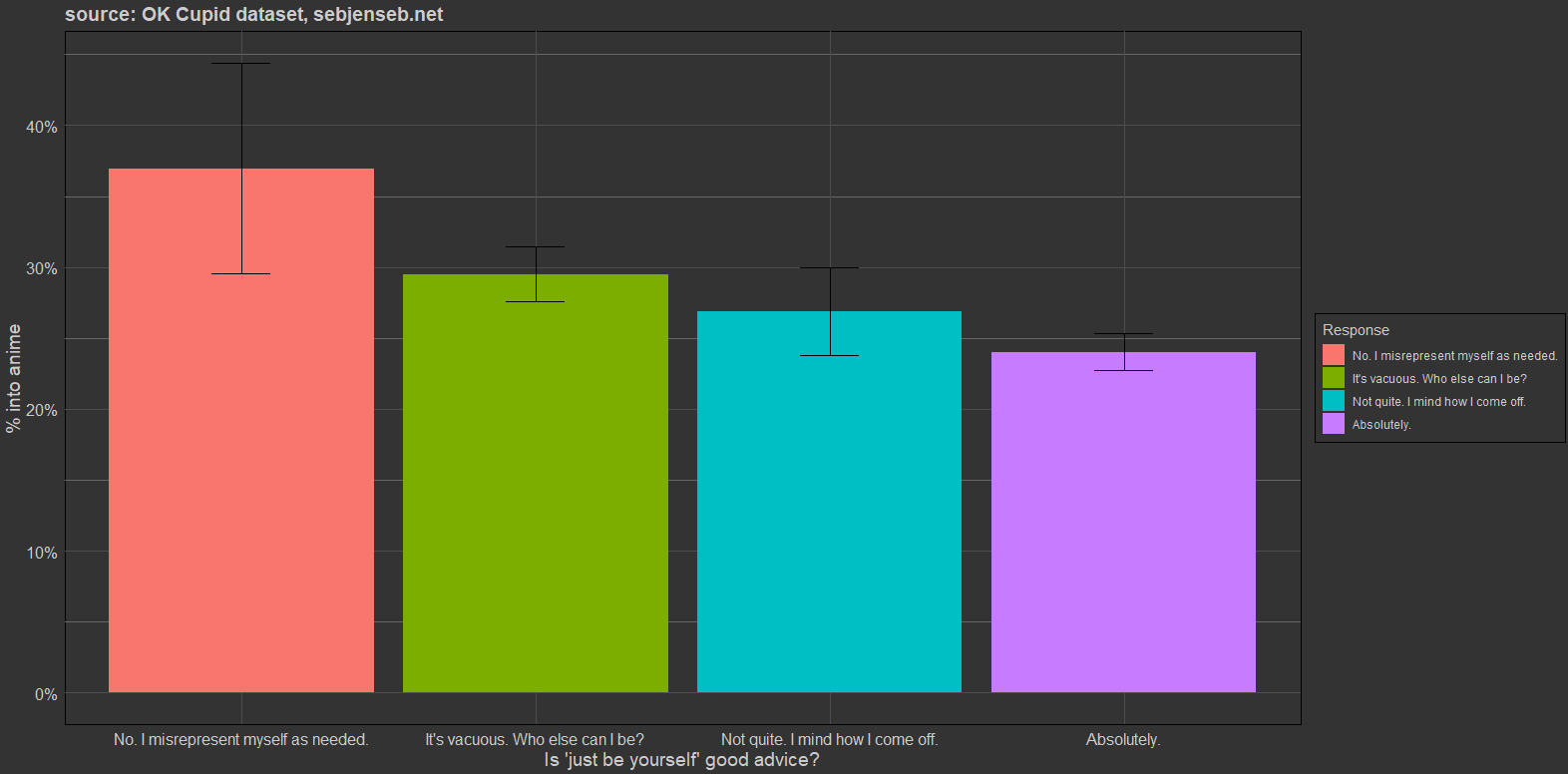
q37545	Is 'just be yourself' good advice?
> okcdataset %>% group_by(q37545) %>% summarise(into_anime = mean(anime, na.rm=T), sum(!is.na(anime)))
# A tibble: 5 × 3
  q37545                               into_anime `sum(!is.na(anime))`
  <chr>                                     <dbl>                <int>
1 Absolutely.                              0.2403                 4307
2 It's vacuous. Who else can I be?         0.2951                 2162
3 No. I misrepresent myself as needed.     0.3697                  165
4 Not quite. I mind how I come off.        0.2690                  803
5 NA                                       0.2507                16355

Carl McNulty

May 23

"TL;DR: people who claim to be really into anime are more likely to be men, childless, poor, bicurious, nonwhite, racist, unathletic, bullied in high school, into Asians, kinky, unconscientious, and eccentric."

Thanks for putting this first, but I could have told you this without any data.

Expand full comment

1 reply

Argos

May 24

It seems like it attracts contrarians to some degree.

17 more comments...

sebjenseb

Discussion about this post