IQ by Chinese Province

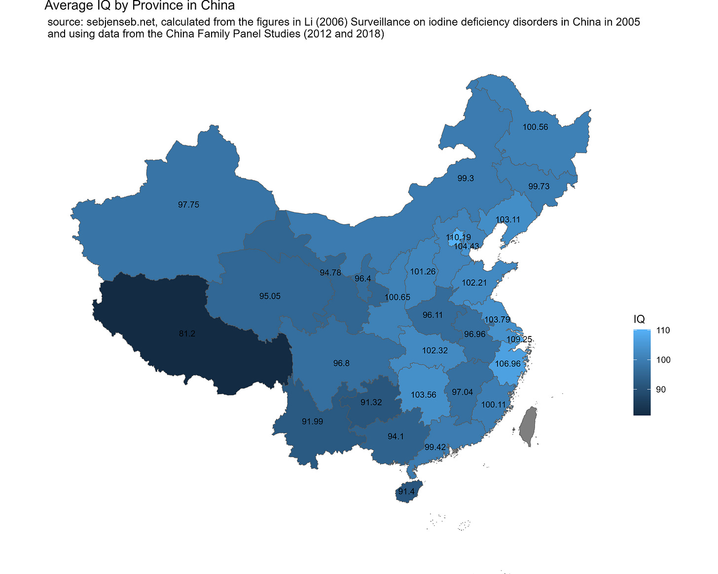
I recently tweeted out a map of the average IQ by Chinese province:

These are based on data collected by some Chinese researchers for an Iodine study.

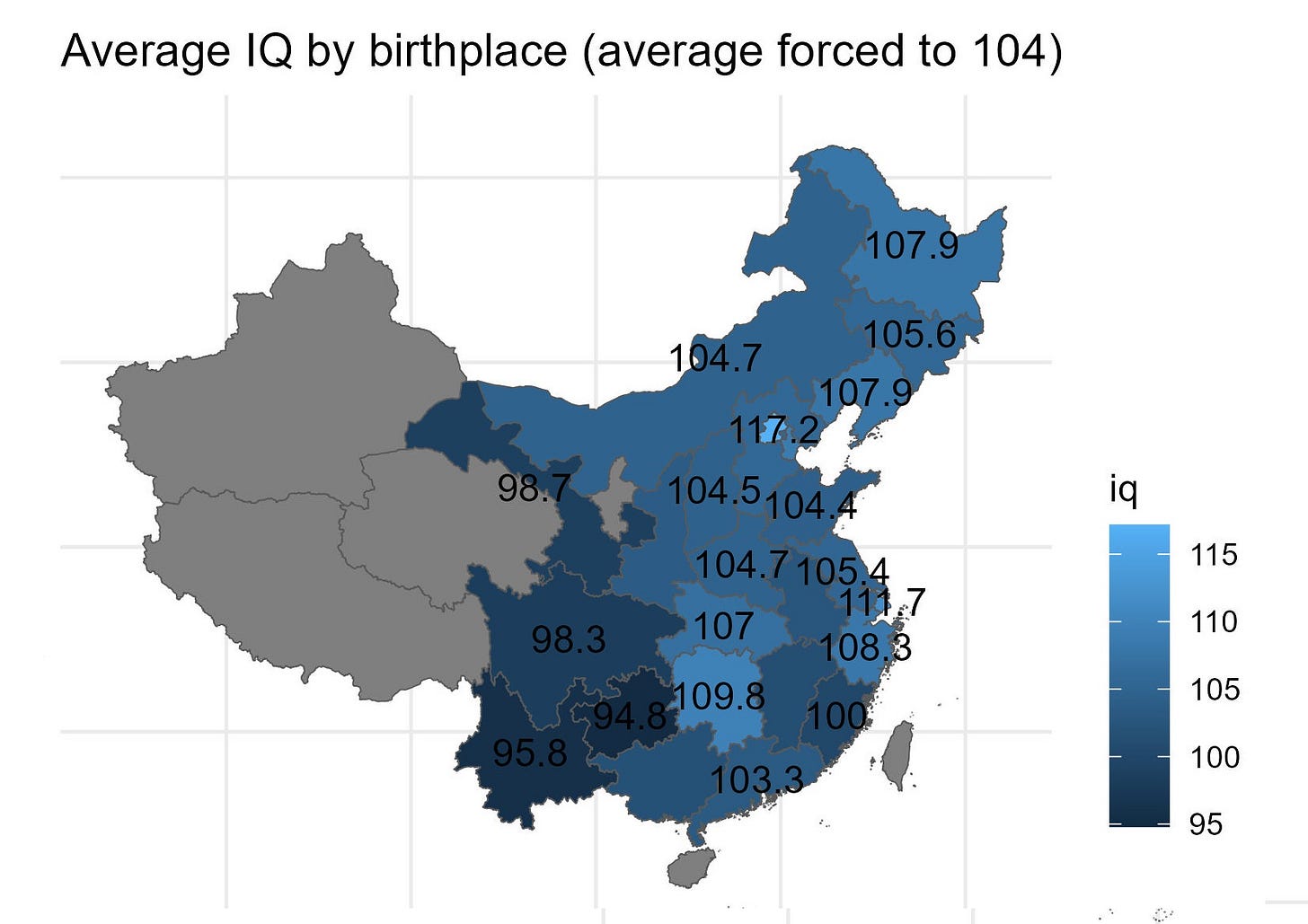
Given that some are skeptical of the Chinese government’s capability to collect this kind of research honestly, I decided to download the CFPS (Chinese NLSY) and tried to estimate the averages myself. I then calculated the average IQ by province and adjusted for selection bias detected within the study using the sampling weights. These were the results:

They correlate at .7 with the results from the iodine study, indicating that there is some consistency to both estimates.

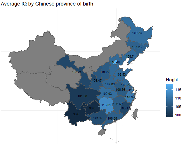
Here’s a second one I made with added number series + memory data:

Code:

chad <- read_sas("C:/Users/_____/OneDrive/Documents/rstuff/thedat.sas7bdat", NULL)

chad$v <- chad$WORDTEST
chad$m <- chad$MATHTEST
chad$age <- chad$QA1AGE
chad$inc <- chad$INCOME
chad$prov <- chad$QA102ACODE

chad$v[chad$v < 0] <- NA
chad$m[chad$m < 0] <- NA
chad$inc[chad$inc < 1] <- NA
chad$age[chad$age < 0] <- NA
chad$schol <- getpc(subset(chad, select=c(v, m)))
#############
fit <- ols(data=chad, as.formula(glue::glue("inc ~ rcs(age, 5)")))
chad$inc2[!is.na(chad$inc) & !is.na(chad$age)] <- fit$residuals
cor.test(chad$inc, chad$inc2)

fit <- ols(data=chad, as.formula(glue::glue("schol ~ rcs(age, 5)")))
chad$schol2[!is.na(chad$schol) & !is.na(chad$age)] <- fit$residuals
cor.test(chad$schol, chad$schol2)
############
cor.test(chad$schol2, chad$inc2)

prov <- unique(chad$prov)
iq <- NA
n <- NA
dante <- data.frame(prov, iq)
dante$n <- n
dante$se <- NA
chad$Rswt_Nat

for(i in 1:length(unique(chad$prov))) {
  j = unique(chad$prov)[i]
  onlyprov <- subset(chad, chad$prov == j)
  dante$n[i] <- nrow(subset(onlyprov, !is.na(onlyprov$schol2)))
  dante$iq[i] <- weighted.mean(x=onlyprov$schol2, weights=onlyprov$Rswt_Nat, na.rm=T)*15+104
  dante$se[i] <- 1/sqrt(nrow(subset(onlyprov, !is.na(onlyprov$schol2))))*15
}


key_list <- list("Beijing" = 11, "Tianjin" = 12, "Hebel" = 13, "Shanxi" = 14, "Inner mongolia" = 15, "Liaoning" = 21, "Jilin" = 22, "Heilongjiang" = 23, "Shanghai" = 31, "Jiangsu" = 32, "Zhejiang" = 33, "Anhui" = 34, "Fujian" = 35, "Jiangxi" = 36, "Shandong" = 37, "Henan" = 41, "Hubei" = 42, "Hunan" = 43, "Guangdong" = 44, "Guangxi Zhuang Autonomous Region" = 45, "Hainan" = 46, "Chongqing" = 50, "Sichuan" = 51, "Guizhou" = 52, "Yunnan" = 53, "Shaanxi" = 61, "Gansu" = 62, "Qinghai" = 63, "Ningxia Hui Autonomous" = 64, "Xinjiang Uygur Autonomous Region" = 65, "Tibet" = 54)

strings <- names(key_list)[match(dante$prov, unlist(key_list))]
print(strings)

dante$snames <- strings

dante$iq[dante$se > 2] <- NA

dante
########
library(maps)
library(rnaturalearth)
library(sf)

china_provinces <- st_read('C:/Users/micha/OneDrive/Documents/rstuff/province.shp')

dante$snames
china_provinces$NAME_PINGY

china_provinces$NAME_PINGY[1] <- dante$snames[4]
china_provinces$NAME_PINGY[2] <- dante$snames[6]
china_provinces$NAME_PINGY[3] <- dante$snames[5]
china_provinces$NAME_PINGY[4] <- dante$snames[11]
china_provinces$NAME_PINGY[5] <- dante$snames[16]
china_provinces$NAME_PINGY[6] <- dante$snames[1]
china_provinces$NAME_PINGY[7] <- dante$snames[22]
china_provinces$NAME_PINGY[8] <- dante$snames[9]
china_provinces$NAME_PINGY[9] <- dante$snames[15]
china_provinces$NAME_PINGY[10] <- dante$snames[2]
china_provinces$NAME_PINGY[11] <- dante$snames[13]
china_provinces$NAME_PINGY[12] <- dante$snames[7]
china_provinces$NAME_PINGY[13] <- dante$snames[27]
china_provinces$NAME_PINGY[14] <- dante$snames[18]
china_provinces$NAME_PINGY[15] <- dante$snames[12]
china_provinces$NAME_PINGY[16] <- dante$snames[17]
china_provinces$NAME_PINGY[17] <- dante$snames[8]
china_provinces$NAME_PINGY[18] <- dante$snames[14]
china_provinces$NAME_PINGY[19] <- dante$snames[19]
china_provinces$NAME_PINGY[20] <- dante$snames[23]
china_provinces$NAME_PINGY[21] <- dante$snames[29]
china_provinces$NAME_PINGY[22] <- dante$snames[20]
china_provinces$NAME_PINGY[23] <- dante$snames[26]
china_provinces$NAME_PINGY[24] <- dante$snames[10]
china_provinces$NAME_PINGY[25] <- dante$snames[32]
china_provinces$NAME_PINGY[26] <- dante$snames[3]
china_provinces$NAME_PINGY[27] <- dante$snames[24]
china_provinces$NAME_PINGY[28] <- dante$snames[31]
china_provinces$NAME_PINGY[29] <- dante$snames[28]
china_provinces$NAME_PINGY[30] <- dante$snames[30]

try <- left_join(china_provinces, dante, by=c('NAME_PINGY' = "snames"))

try$centroid <- st_centroid(try$geometry)

ggplot(data = try) +
  geom_sf(aes(fill = iq)) +  # Assuming the column with province names is named "NAME"
  theme_minimal() +
  geom_sf_text(aes(label = round(iq, 1), geometry = centroid), check_overlap = TRUE, size=3) +
  labs(title = "Average IQ by birthplace (average forced to 104)", fill = "iq") +
  theme(axis.text.x = element_blank(), 
        axis.text.y = element_blank(),
        axis.ticks = element_blank())