

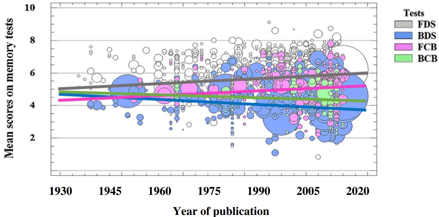
I identified one major error in a study on the Flynn Effect that I had frequently cited prior. It meta-anlyses performance on the number of digits one can memorise (digit span) forwards and backwards across time, finding that performance on forward digit span improved over time, but performance in backwards digit span worsened:

The Flynn effect has been investigated extensively for IQ, but few attempts have been made to study it in relation to working memory (WM). Based on the findings from a cross-temporal meta-analysis using 1754 independent samples (n = 139,677), the Flynn effect was observed across a 43-year period, with changes here expressed in terms of correlations (coefficients) between year of publication and mean memory test scores. Specifically, the Flynn effect was found for forward digit span (r = 0.12, p < 0.01) and forward Corsi block span (r = 0.10, p < 0.01). Moreover, an anti-Flynn effect was found for backward digit span (r = − 0.06, p < 0.01) and for backward Corsi block span (r = − 0.17, p < 0.01). Overall, the results support co-occurrence theories that predict simultaneous secular gains in specialized abilities and declines in g. The causes of the differential trajectories are further discussed.
This is relevant because the ability to memorise digits backwards is a better indicator of intelligence than the ability to memorise them forwards, so it has been cited as evidence that the Flynn Effect is an artefact of performance changes on specific tests instead of a general improvement in cognition.
I downloaded their data out of curiosity and decided to check for errors. I found one in their 2nd regression table, where I was unable to replicate the statistically significant1 decline in backwards digit span over time.
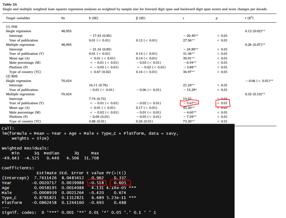
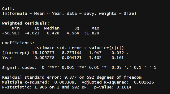
I was otherwise able to replicate the other coefficients in their model, like the intercept being 7.74 or the effect of country being 0.88, so I’m inclined to think the failure to replicate is not a function of small differences in underlying data or methodology. I was also similarly able to replicate the paramaters in their zero-order regression (16.11 and -0.01) but not the p-values and t-statistics2.
The table is otherwise strange. One intercept is listed as statistically significant (24.89) and another is not (10.52) despite both having large t-statistics. They have one t-statistic listed with one star (15.29) but explicitly labelled as < .01 in the table, which is odd as they claim in Table 2B that one star is only p < .05.
Essentially, my claim is that they made a mistake somewhere along the way and found a null to be a positive finding. If they were fraudulent researchers, they probably would not bother sharing their data.
Doing things my way
Different age groups have different standard deviations in terms of digit span, so this must be adjusted for when calculating the change in performance over time. As the averages may also vary by country, I categorised every single one of the effect sizes by country (all 592!) by searching for the publication using the author/year that they gave. In 22 instances I could not find the original source. I also added a few other uncited publications along the way, bringing up the total number of effect sizes to 599. I also labelled the perceived SES of the sample (higher for professional workers or college students, average for high school students or volunteers, low for unskilled labourers). I weighed by the square root of the sample size instead of the raw number, as that is standard practice.
Fitting a spline to the data and controlling for age/SES/country3 suggested that backward digit span has increased by about 5.5 IQ points (41 x 0.13518) over the 1975 - 2016 time period. The effect was statistically significant4, but not to an impressive degree (p = .0063).
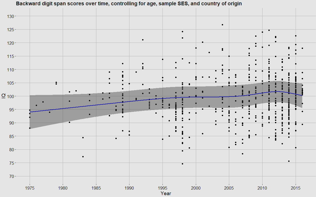
The spread of scores is high because the data is not of particularly high quality. The age-norming and country categorising were attempts to remedy this, but unfortunately they only provided marginal improvements.
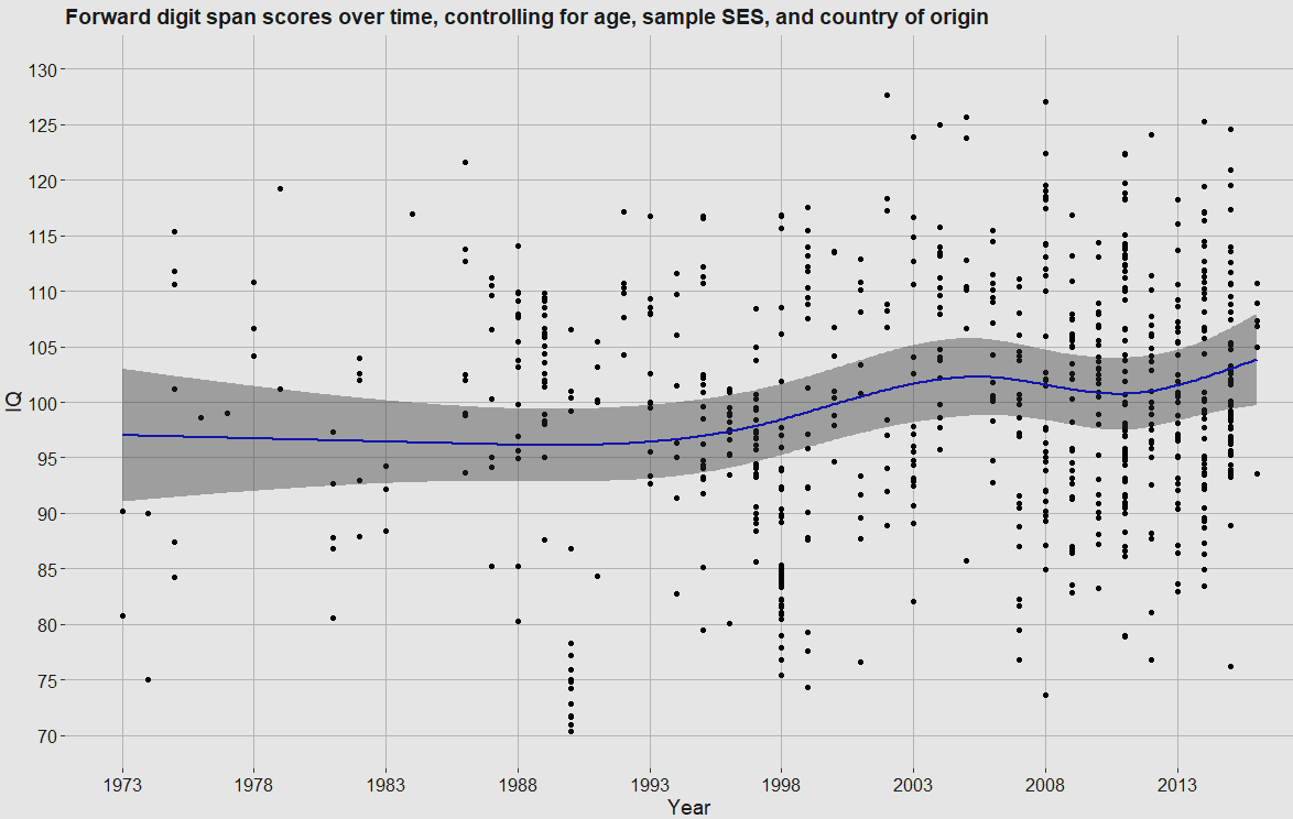
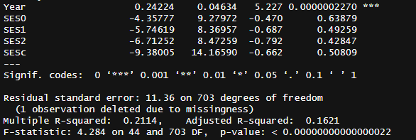
It would also be prudent to test whether the same holds in the forward digit span test. It did, with a larger effect (9.9 points) and a much more clear effect (p = .00000023)5.
In all
Both of the increases over time are statistically significant and of similar magnitudes, which leads me to believe that this particular criticism of the Flynn Effect is not valid. I am still skeptical that observed Flynn Effect gains represent true gains in intelligence, though I don’t think this publication and data should be cited as being evidence against the intelligence-gain hypothesis, and my priors have shifted slightly towards FE gains reflecting some increases in real intelligence.
I have the code6 I used, but it’s not very useful because I use a lot of proprietary functions to run it. It’s also illegible because I wrote it for my own purposes. I do have the dataset I used to make my own calculations on the alternative website, which is more useful.
That is to say, their decline in backwards digit span over time was far more extreme in comparison to what would be expected from chance if it was not the case that there was no change over time.
Table:
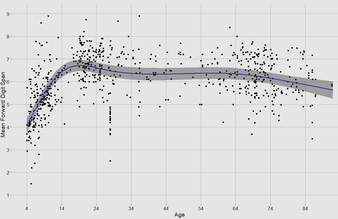
Relevant charts:
Mean(Score) ~ Age, controlled for year/country/SES. Peak is 19.5.
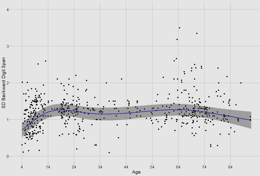
SD(Score) ~ Age, controlled for year/country/SES

Same charts but backwards:
Peak is 22.5
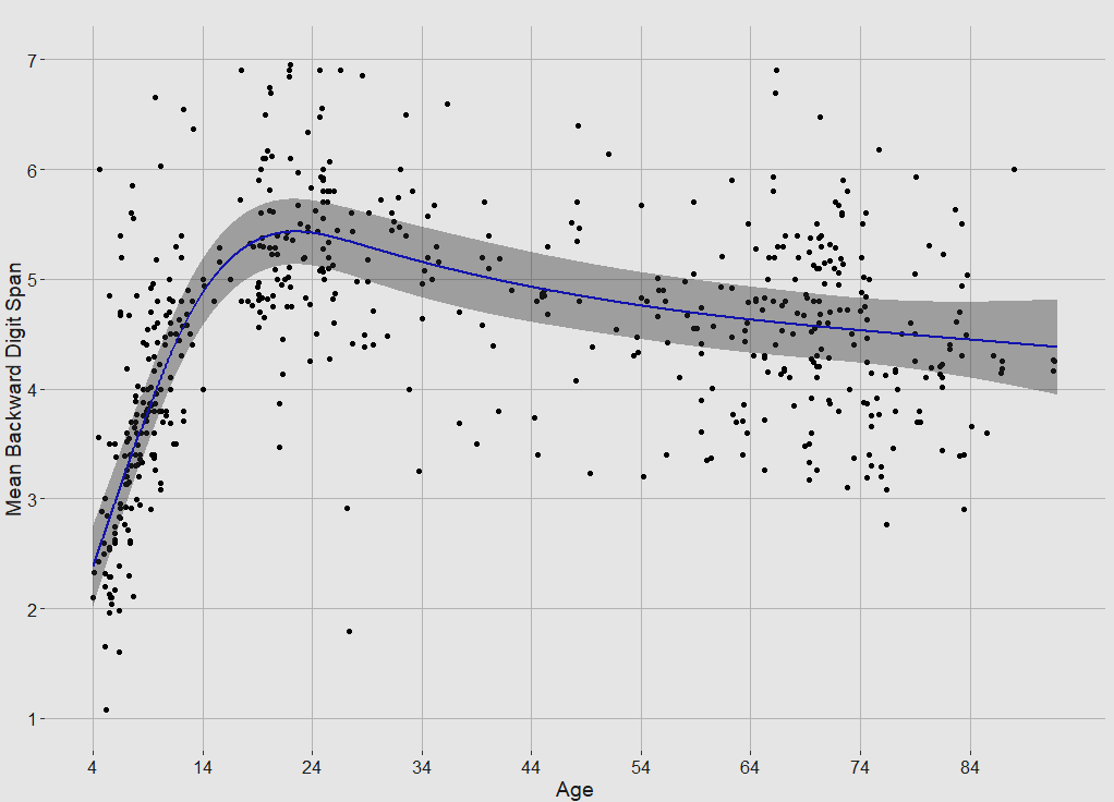
Table:
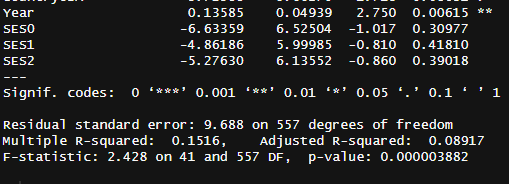
Table:
qwe <- lm(data=savy, Mean ~ Year, weights=Size)
summary(qwe)

qwe <- lm(data=savy, Mean ~ Year + Age + Male + Type_C + Platform, weights=Size)
summary(qwe)

################
testtempyarfwefe <- allspan


subset <- testtempyarfwefe %>% filter(type==’backward’)
subset$Country[is.na(subset$Country)] <- ‘Unknown’
subset$SES[is.na(subset$SES)] <- 1
subset$SE <- subset$SD/sqrt(subset$Size)
subset$Country[(subset$Country==1 | subset$Country==0 | subset$Country==’‘)] <- ‘Unknown’
unique(subset$Country)

p <- splinechart(datos=subset, var1=’Age’, var2=’Mean’, knots=5, breakn=10, metastyle=F, label=’Age’, labely=’Mean Backward Digit Span’,
                 covariatefunc=’ + as.factor(SES) + Year + Country’, ws=’Size’, burndata=data.frame(SES=1, Country=’UK’, Year=2000), outputyes=F)
p

p <- splinechart(datos=subset, var1=’Age’, var2=’Mean’, knots=5, breakn=10, metastyle=F, label=’Age’, labely=’Mean Backward Digit Span’,
                 covariatefunc=’ + as.factor(SES) + Country’, ws=’Size’, burndata=data.frame(SES=1, Country=’UK’), outputyes=F)
p

#Yes, this does pass significance testing
p <- splinechart(datos=subset, var1=’Age’, var2=’SD’, knots=5, breakn=10, metastyle=F, label=’Age’, labely=’SD Backward Digit Span’,
                 covariatefunc=’ + as.factor(SES) + Country + Year’, ws=’Size’, burndata=data.frame(SES=1, Country=’UK’, Year=2000), outputyes=F)
p

lr <- lm(data=subset, Mean ~ rcs(Age, 5) + as.factor(SES), weights=sqrt(Size))
summary(lr)
metaobj2 <- metafor::rma(yi=Mean, sei=SE, data=subset, mods = ~ rcs(Age, 5) + as.factor(SES))
summary(metaobj2)
lr$coefficients <- metaobj2$b

metaobj32 <- metafor::rma(yi=SD, sei=SE, data=subset, mods = ~ rcs(Age, 5) + as.factor(SES))
summary(metaobj2)
lr3 <- lm(data=subset, SD ~ rcs(Age, 5) + as.factor(SES), weights=sqrt(Size))
summary(lr)
lr3$coefficients <- metaobj32$b

uzi <- seq(from=4, to=92.5, by=.1)
uzi2 <- data.frame(Age=uzi, SES=1)
uzi2$SD_age = predict(lr3, uzi2)

subset$residualscore <- lr$residuals
subset$roundage <- format(round(subset$Age, 1), nsmall = 1)
uzi2$Age_formatted <- format(uzi2$Age, nsmall = 1)

subset2 <- left_join(
  subset,
  uzi2 %>% select(Age_formatted, SD_age),
  by = c(’roundage’ = ‘Age_formatted’)
)

subset2$IQ <- subset2$residualscore/subset2$SD_age*15+100

p <- splinechart(datos=subset2, var1=’Year’, miny=70, maxy=130, var2=’IQ’, knots=5, breakn=5, breakny=5, metastyle=F, label=’Year’, labely=’IQ’, titul = ‘Backward digit span scores over time, controlling for age, sample SES, and country of origin’,
                 covariatefunc=’+ Country + as.factor(SES) + Year’, ws=’Size’, burndata=data.frame(SES=1, Country=’UK’, Year=2000), outputyes = T)
p

lr <- lm(data=subset2, IQ ~ Country + Year + SES)
summary(lr)

41*0.13585


#################################

burndata <- data.frame(
  SES = 1,
  Country = ‘UK’,
  Year = 2000
)

uzi2 <- seq(from=18, to=30, by=0.1)

covariatefunc=’‘

modelt = paste0(’ ‘)
lr <- lm(data=subset, Mean ~ rcs(Age, 5) + as.factor(SES) + Year + Country, weights=sqrt(Size))
summary(lr)


uzi2 <- seq(from=18, to=30, by=.1)
uzi4 <- data.frame(Age=uzi2, burndata)

# Predict
uzi4$fit <- predict(lr, newdata=uzi4, interval=”confidence”)

uzi4


##################
###############
testtempyarfwefe <- allspan

subset <- testtempyarfwefe %>% filter(type==’forward’)
subset$Country[is.na(subset$Country)] <- ‘Unknown’
subset$SES[is.na(subset$SES)] <- 1
subset$SE <- subset$SD/sqrt(subset$Size)
subset$Country[(subset$Country==1 | subset$Country==0 | subset$Country==’‘)] <- ‘Unknown’
unique(subset$Country)

p <- splinechart(datos=subset, var1=’Age’, var2=’Mean’, knots=5, breakn=10, metastyle=F, label=’Age’, labely=’Mean Forward Digit Span’,
                 covariatefunc=’ + as.factor(SES) + Year + Country’, ws=’Size’, burndata=data.frame(SES=1, Country=’UK’, Year=2000), outputyes=F)
p

p <- splinechart(datos=subset, var1=’Age’, var2=’Mean’, knots=5, breakn=10, metastyle=F, label=’Age’, labely=’Mean Forward Digit Span’,
                 covariatefunc=’ + as.factor(SES) + Country’, ws=’Size’, burndata=data.frame(SES=1, Country=’UK’), outputyes=F)
p

#Yes, this does pass significance testing
p <- splinechart(datos=subset, var1=’Age’, var2=’SD’, knots=5, breakn=10, metastyle=F, label=’Age’, labely=’SD Forward Digit Span’,
                 covariatefunc=’ + as.factor(SES) + Country + Year’, ws=’Size’, burndata=data.frame(SES=1, Country=’UK’, Year=2000), outputyes=F)
p

lr <- lm(data=subset, Mean ~ rcs(Age, 5) + as.factor(SES), weights=sqrt(Size))
summary(lr)

metaobj2 <- metafor::rma(yi=Mean, sei=SE, data=subset, mods = ~ rcs(Age, 5) + as.factor(SES))
summary(metaobj2)
lr$coefficients <- metaobj2$b

metaobj32 <- metafor::rma(yi=SD, sei=SE, data=subset, mods = ~ rcs(Age, 5) + as.factor(SES))
summary(metaobj2)
lr3 <- lm(data=subset, SD ~ rcs(Age, 5) + as.factor(SES), weights=sqrt(Size))
summary(lr)
lr3$coefficients <- metaobj32$b

uzi <- seq(from=4, to=92.5, by=.1)
uzi2 <- data.frame(Age=uzi, SES=1)
uzi2$SD_age = predict(lr3, uzi2)

subset$residualscore <- lr$residuals
subset$roundage <- format(round(subset$Age, 1), nsmall = 1)
uzi2$Age_formatted <- format(uzi2$Age, nsmall = 1)

subset2 <- left_join(
  subset,
  uzi2 %>% select(Age_formatted, SD_age),
  by = c(’roundage’ = ‘Age_formatted’)
)

subset2$IQ <- subset2$residualscore/subset2$SD_age*15+100

p <- splinechart(datos=subset2, var1=’Year’, var2=’IQ’, maxy=130, miny=70, knots=5, breakn=5, breakny=5, metastyle=F, label=’Year’, labely=’IQ’, titul = ‘Forward digit span scores over time, controlling for age, sample SES, and country of origin’,
                 covariatefunc=’+ Country + as.factor(SES) + Year’, ws=’Size’, burndata=data.frame(SES=1, Country=’UK’, Year=2000), outputyes = T)
p

lr <- lm(data=subset2, IQ ~ Country + Year + SES)
summary(lr)

41*0.2422


#################################


burndata <- data.frame(
  SES = 1,
  Country = ‘UK’,
  Year = 2000
)

uzi2 <- seq(from=18, to=30, by=0.1)

lr <- lm(data=subset, Mean ~ rcs(Age, 5) + as.factor(SES) + Year + Country, weights=sqrt(Size))
summary(lr)


uzi2 <- seq(from=18, to=30, by=.1)
uzi4 <- data.frame(Age=uzi2, burndata)

# Predict
uzi4$fit <- predict(lr, newdata=uzi4, interval=”confidence”)

uzi4