
Meta-analysis of 1250 correlations between family members in phenotypes

Between the Minnesota study of twins reared apart, Haworth’s meta-analysis of twin studies of intelligence, the Dutch twin study, Segal’s twins reared apart, Bouchard’s tables of correlations between family members in IQ1, Burt’s study of family members reared apart2, the Korean-American study of adoptees, the Brothers sample, Hyytinen’s meta-analysis of twin studies on income, Horwtiz’s meta-analysis of assortative mating, the Swedish Adoption/Twin Study of Aging (which I analyzed), Jelenkovic’s meta-analysis of twin studies on height, Hatemi’s meta-analysis of twin studies on political views, Elks et al meta-analysis of BMI, the Finnish study of twins reared apart, and dozens of other publications, I’ve assembled 1250 correlations between family members in traits, representing about 170,000,000 pairs of individuals. The dataset is available here3.
I tracked several moderators, including the reliability of the measure, the age of the sample, the year the subjects were tested, and the nation in which the data was collected. Sometimes, the exact age of the sample could not be calculated and had to be inferred based on the context, so some samples were labelled as being “dependents”, “adults”, or “all ages”. Samples with measurable ages were labelled as “adult” if all subjects were above 16, “dependents” if all subjects were below 16, or of “all ages” if they did not satisfy either of those criteria. The mean age for each of those age category was imputed into those who did not have measurable ages. This process was carried out within traits, as the average age of testing varies by trait. Given the high average ages at testing, these heritability estimates should be considered appropriate for adults.
To be included in the sheet, studies had to show sample sizes for each kin correlation and not overlap with data from any other study. If no test reliability data was available, the median reliability was used as an estimate, and if no year at testing was available, the publication year minus two years was used as a guess.
In all cases, I meta-analyze the kin correlations by running a random effects meta-analysis within each category.
After reviewing the traits individually, I have come to these conclusions:
In graphic form:
These are the trait correlations within adults:
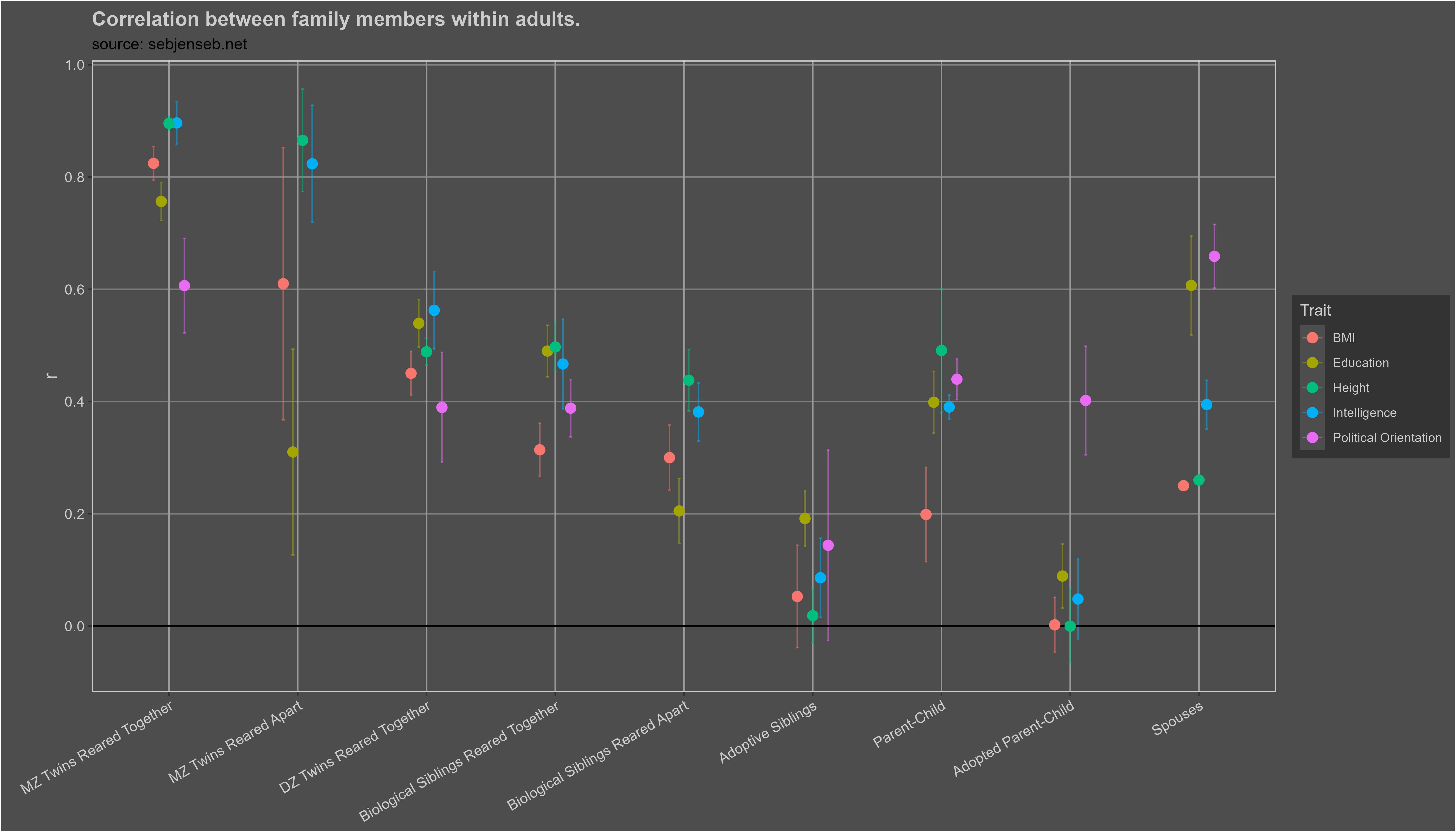
I found zero (0) evidence of phenotypic transmission from parent to child for every single trait except for political orientation, education, income, and wealth. In the case of political orientation, the effect is very large: about 5-10%4 of an individual’s political orientation can be explained by non-genetic transmission from a parent to their child; in the case of education, income, and wealth, these figures are 2%, 5%5, and 6% respectively. I suspect these effects are due to environmental confounding; the environments that parents grow up in correlate with those that their children grow up, so correlations between parents and children will be observed, even if they are not genetic or cultural in nature. The relationships are also coincidentally observed in traits with large shared environmental effects, which would be expected if the correlations were an artefact of environmental confounding.
These figures could also arise due to environmental confounding; the environments that parents grow up in correlate with those that their children grow up in, as such, evidence of phenotypic transmission is observed without the existence of true phenotypic transmission.
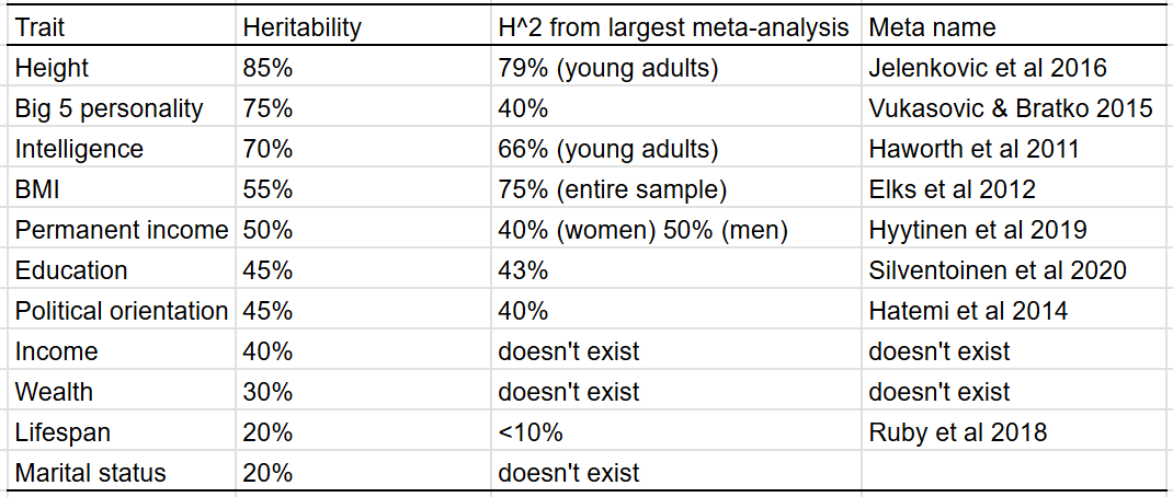
I compared the heritability estimates I estimated to those found by other researchers6 for the purposes of external validity. In most cases, my estimates agreed with that of the academic literature, with the exceptions of lifespan, personality, and BMI.
Changelog:
First round of edits7
Heritability modelling
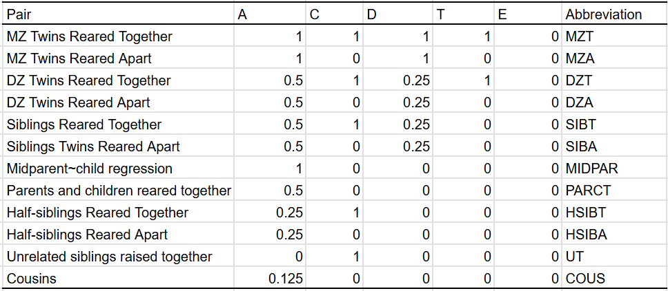
In most cases, I have the privileges of having many different types of family members, so I can plug them all into a statistical model that estimates a set of parameters. In the traditional twin model, these are A (additive genes), C (shared environment), and E (unshared environment). When appropriate, I estimate D (dominant genes) and T (twin-specific effects). These are the similarities between family pairs in each component:
In the event that there are violations in the EEA assumption (that MZ twins are equal in environments relevant to the trait relative to DZ twins)8, epistatic effects9 (interactions between genetic locations), imperfect correlations between genetic factors between generations10, or non-linear interactions between genes and environmental factors11, those sources of variance will be shuffled to the dominant component in the model. Given that the search for dominance/epistasis in molecular genetics has been a massive disappointment, priors dictate that variance explained by the dominant component is not actually dominance.
If it’s the case that epistasis is occuring, or if there are imperfect correlations between genetic effects between generations, then the bias is a non-issue, as the dominant component is picking up on another source of genetic variance. However, if it’s picking up on violations due to EEA violation or non-linear interactions between genes and environmental factors, then that is a problem because those are not genetic sources of variance.
In some cases I adjust for assortative mating, which inflates the genetic relationship between relatives. I do this by plugging an assumed narrow-sense heritability and correlation between spouses into the variance components:
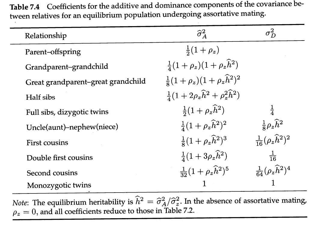
For example, if spouses correlate at .6 in educational attainment, then the additive coefficient for the correlation between parents and children is 0.8, not 0.5.
I have to simulate data to run these models; I do this by using a selfmade R function that generates sets of family pairs that correlate at a given value. If this is done using base R, the correlation is imprecise; e.g. if you instruct it to generate a set of 100 pairs of datapoints that correlate at 0.6, they will not correlate at exactly 0.6 because of random error. I get past this by instructing R to simulate data until the observed correlation is within a desired boundary (usually 0.0001). I also set the sample size to the one that would be inferred from the standard errors estimated from the random-effects meta-analysis to avoid heterogeneity from biasing the estimation of standard errors.
Usually I don’t report CIs because the dataset is so massive that the SEs for the variance components are typically lower than 1%, even with the heterogeneity adjustments:
My takeaways from the study:
Everything is heritable (1st law)
For the average trait, environmental influences are equal to genetic ones.
Traits differ substantially in their heritability.
All traits with a heritability under 100% are influenced by the shared environment.
Most traits have twin-specific effects or sex-specific effects.
Heritability estimation methods using different family members or variance components tend to be consistent.
Phenotypic transmission from parents to children is rare.
Intelligence — heritability of 70% (60%-80%)
I adjusted each correlation for test reliability12, and assumed a reliability of .91 if a study did not publish the reliability of its test. Here I plot the correlations within all individuals:
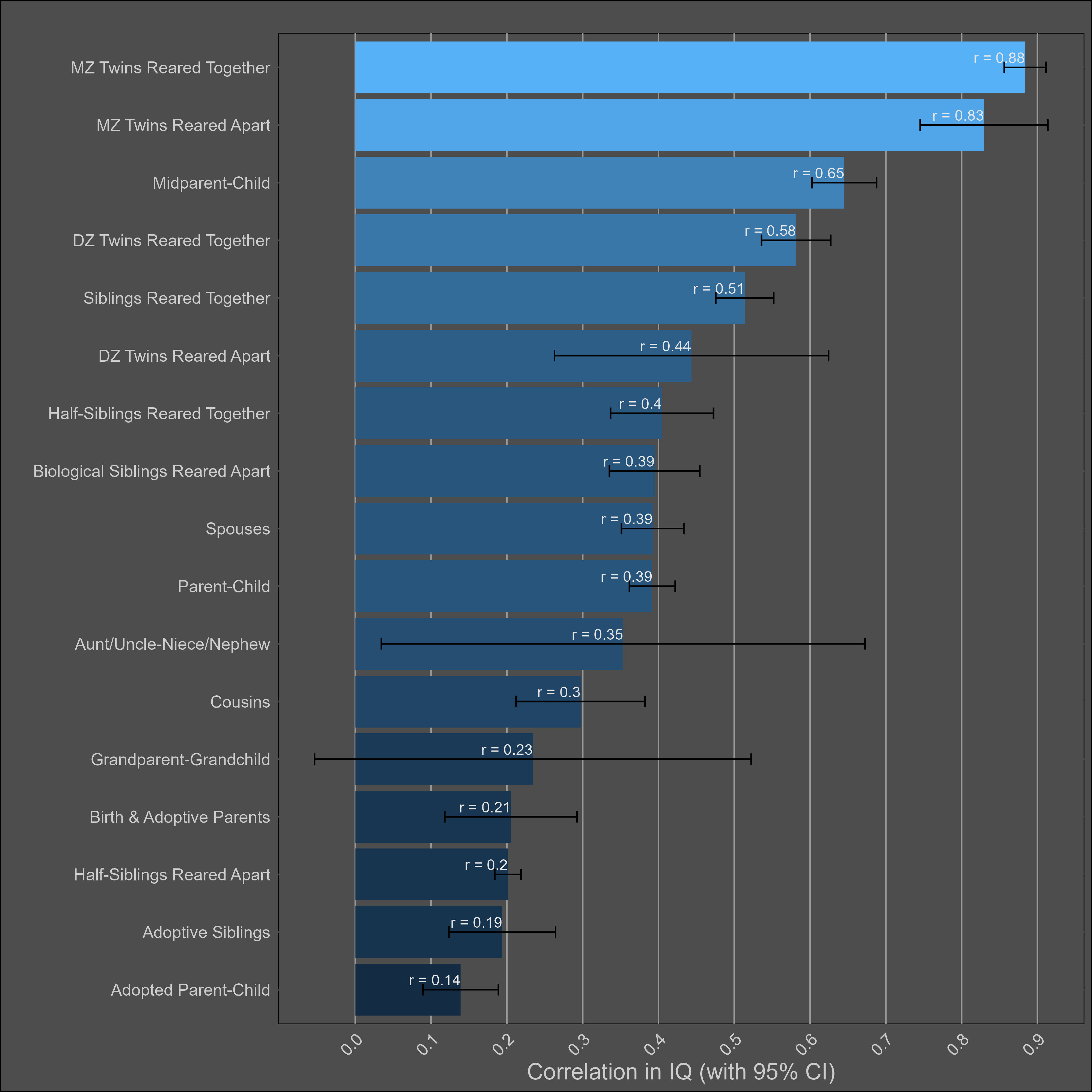
Visually, I see a high heritability, a small shared environmental effect, and no cultural transmission of intelligence. I found no evidence of publication bias13 in any of the 17 correlations.
The observed correlation between adoptive parents and their children is mostly due to selective placement. Given that birth and adoptive parents correlate at .21, and that biological parents and children correlate at .39, one would expect adoptive parents and their children to correlate at 0.082 (.21 x .39), which is close to the observed correlation (.14). The relationship is also not statistically significant within adults.
There are various ways one can calculate the hertiability of intelligence using this data — the most simple is measuring the correlation in identical twins reared apart, which mathematically turns out to be an estimate of the heritability of a trait; others include averaging the trait values of the parents and regressing them on a single child, which computes the narrow sense heritability (variance in phenotype that can be attributed to additive genetic variation
There are two methods one can use to estimate the shared environmental component without formal modelling: one is simply computing the correlation between unrelated siblings, the other is computing the difference between family members reared apart and together with the same genetic relationship.
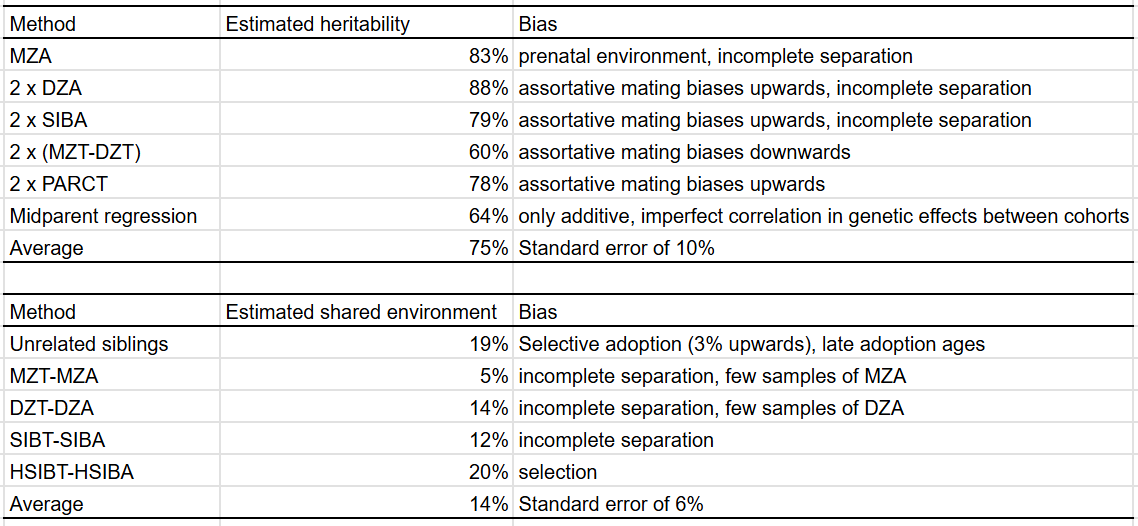
As expected, the methods with upwards bias (MZA, 2xDZA/SIBA/PARCT) all have high heritability estimates, and the ones with downwards biases (falconer formula, midparent regression) have lower ones. The T-A methods diverge, but on average are close to the method of using unrelated siblings.
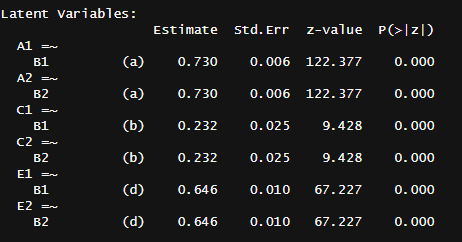
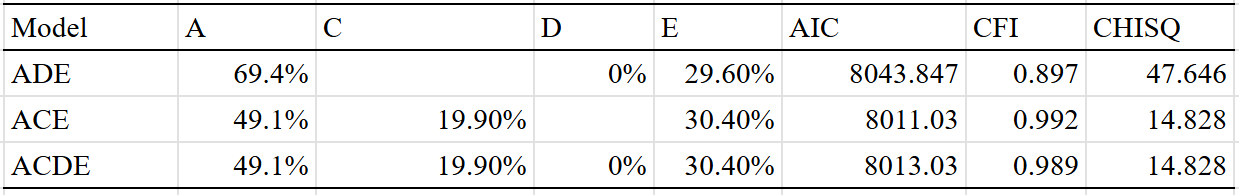
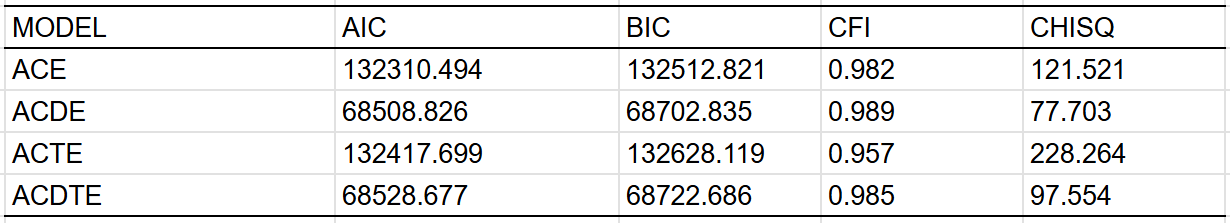
I also used formal statistical modelling to estimate trait heritability. These were the results:
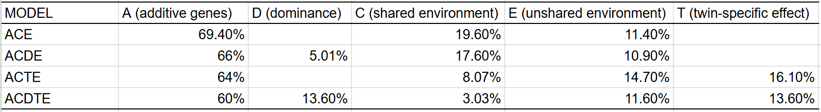
The model with the best fit14 was ACDE, though there does seem to be a small twin-specific effect, judging by the higher correlation between DZ twins than siblings. Given that midparent ~ child regression shows that the narrow sense heritability of IQ is 60-70% (even in young adults), all heritability above that number must be non-additive: epistasis, dominance, or GxE. Given that we have good reason to think those are negligible sources of variance, I am reticent to estimate a heritability of intelligence far above this number.
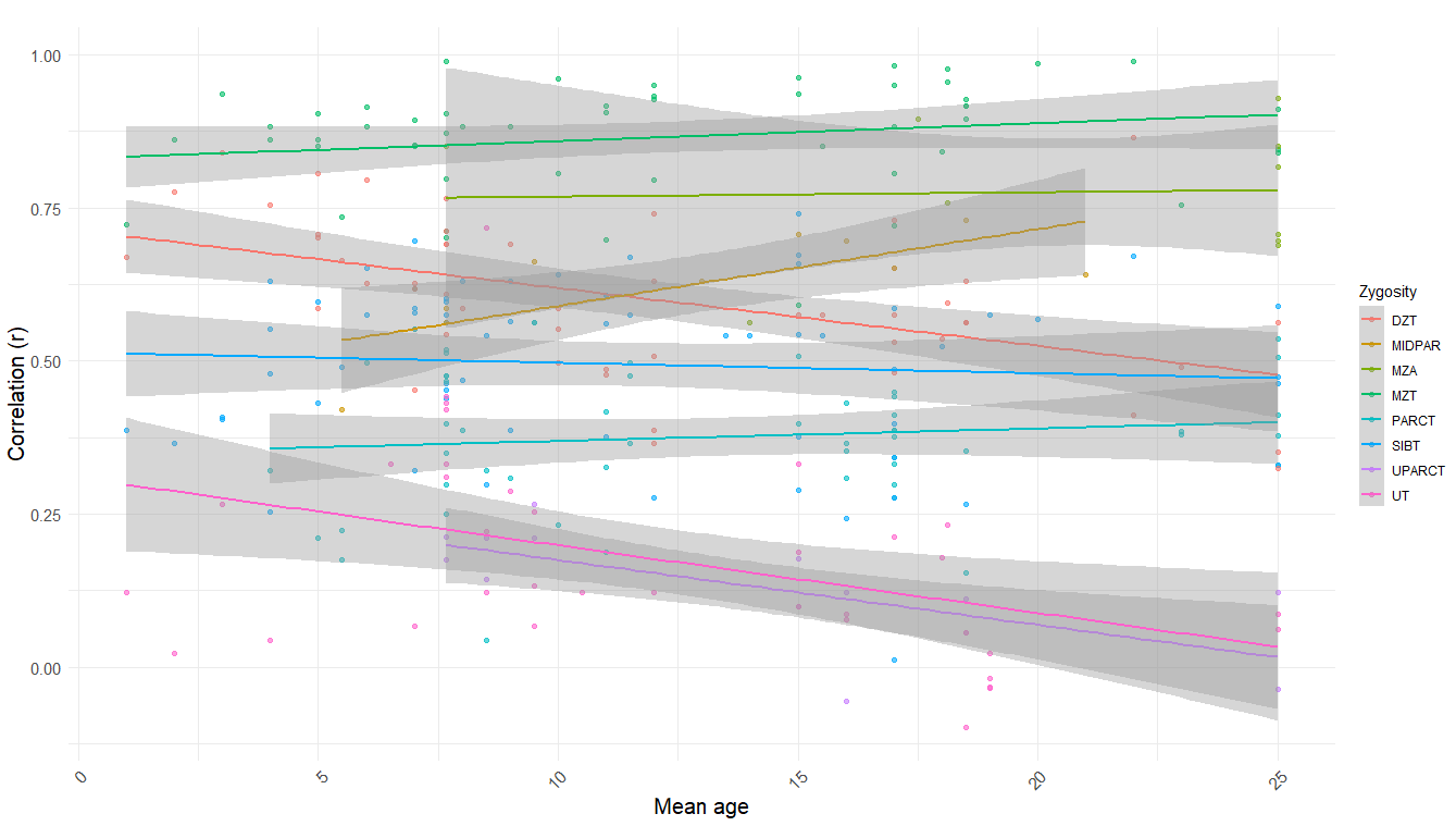
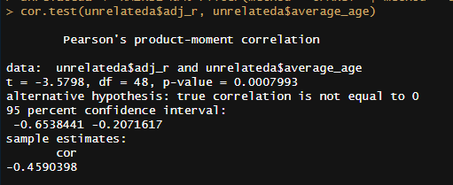
In terms of age trends, the only statistically significant trend was that in DZ twins reared together, dropping from ~.6 in childhood to ~.5 in adulthood. When pooled together, there is a strong negative correlation (r = -.46, p < .001)15 between mean age and relatedness in samples of unrelated individuals reared together (UPARCT and UT).
It’s a myth that C^2 = 0 in adults; Cesarini found that scores of genetically unrelated siblings on the Swedish military entrance exam, taken at the age of about 18, correlate at .17 (n = 1,647 individuals). We also have not found any trait with a shared environmental effect of zero that has a heritability of below 100%, so our priors for this being the one are, well, low.
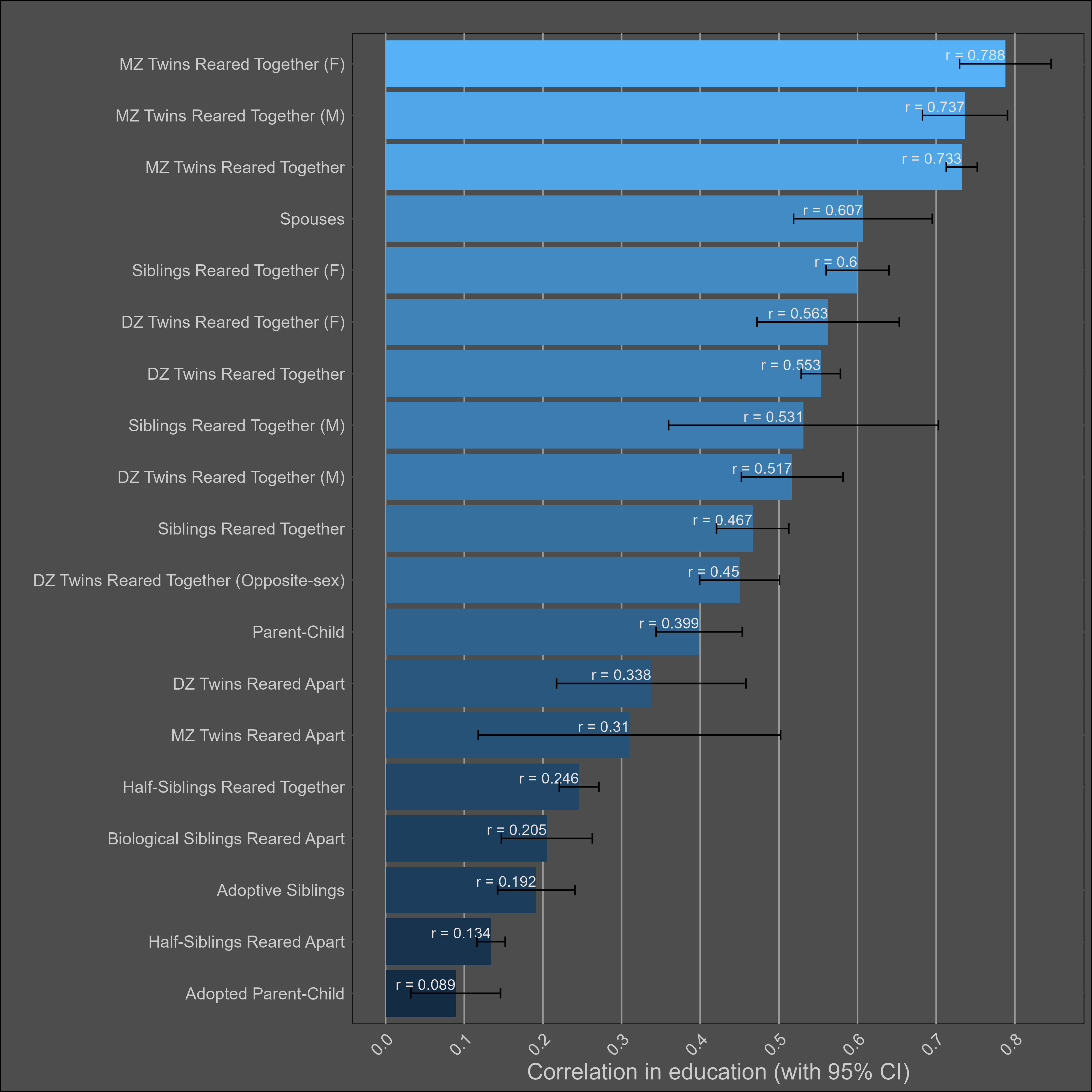
Education — 45% (40% - 50%)
The plot:
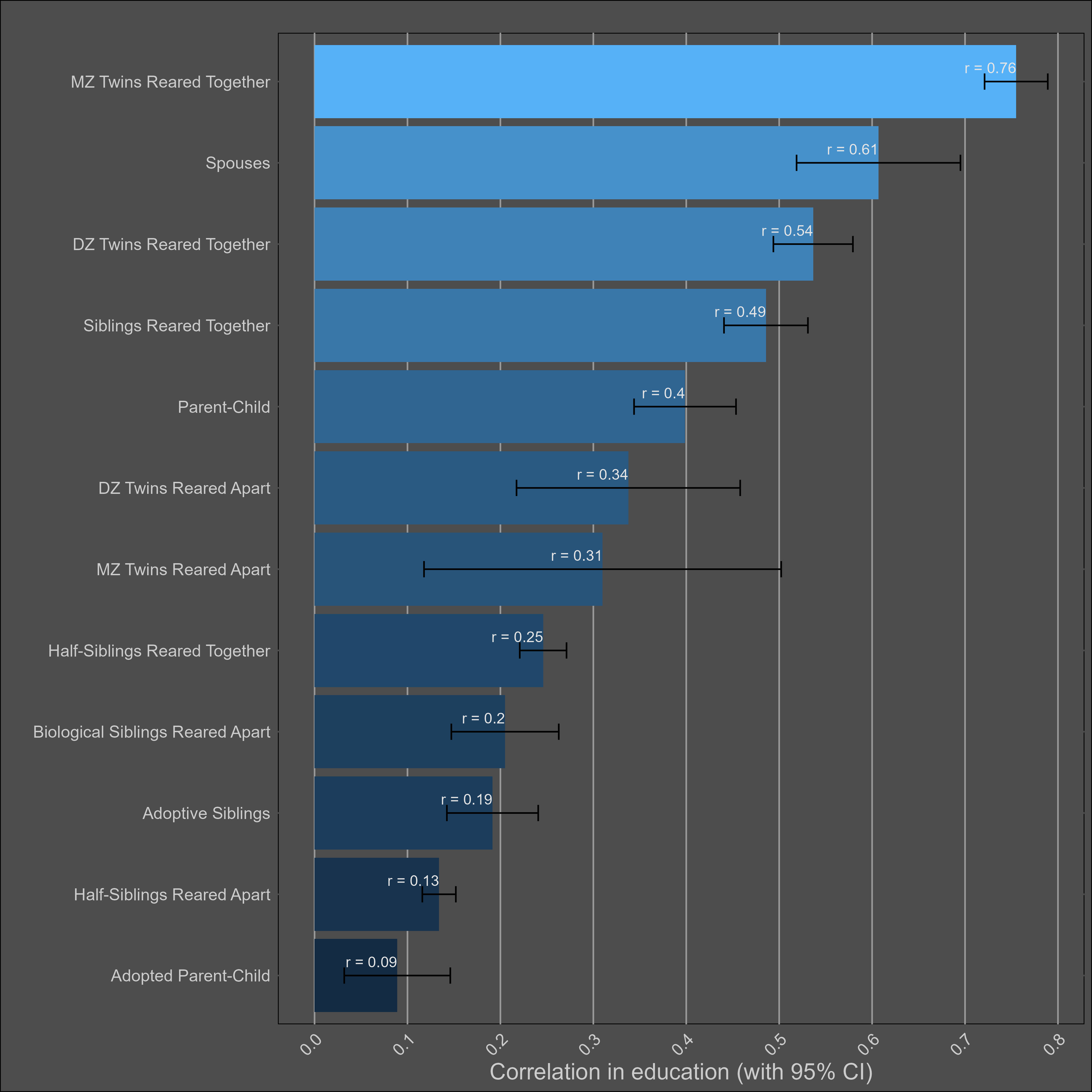
Transmission from adoptive parents to children is statistically significant, but a non-factor; even if the correlation between adoptive parents and their children is generously estimated to be 0.15, that would imply that 4% of the variance in children’s education is due to transmission from child to parent16. In contrast, the parent~child correlation in education suggests that the narrow sense heritability is 39%17, biased downwards by imperfect correlations in genetic effects between cohorts.
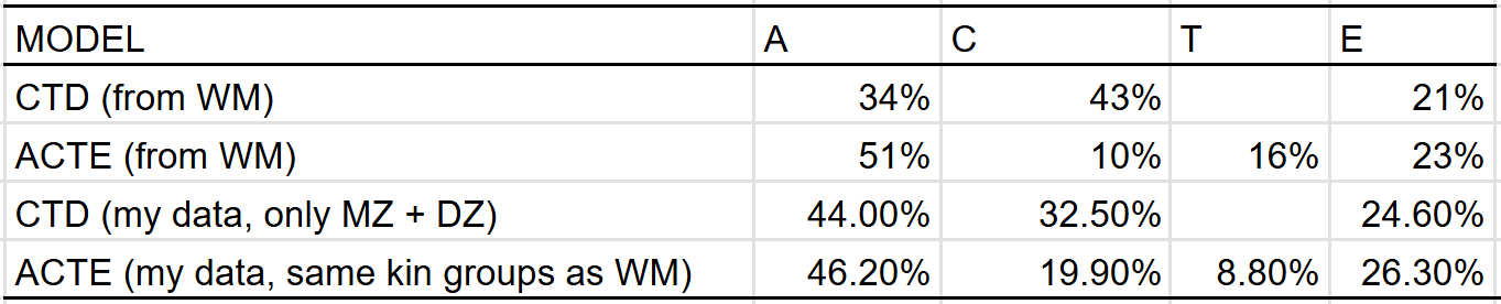
The existence of C (shared environmental) and T (twin-specific) effects is a given, so all of the models I ran included these effects. I set the sample size of the sample of half-siblings reared apart to be the same as the average for all methods (1500) and subtracted the correlation between parents and children by 0.09 to adjust for direct phenotypic transfer. I then ran six different models, varying by the extent to which they corrected for assortative mating or included dominance.
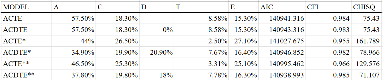
The dominant effects are too large to be credible, and are likely capturing other effects; as such I am liable to trust the additive-only models which estimate a heritability of 44-46% for educational attainment. It’s possible that the true broad-sense heritability is up to 60% based on the (on paper, better fitting) ACDTE models, but I’ll have to see it to believe it.
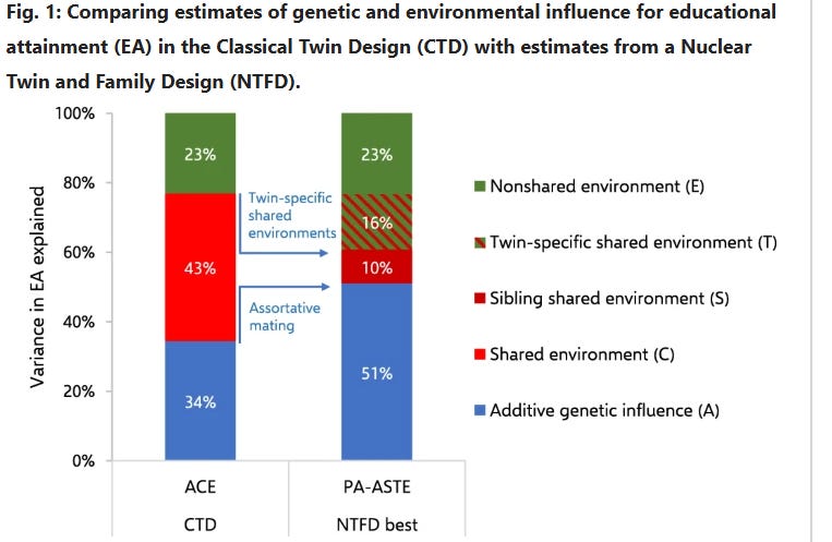
The C^2 and T^2 effects that I estimate differ from those made by Wolfram & Morris, who estimated that the effect of the shared environmental component decreased from 43% to 10% when adjusting for twin-specific effects. This could be due to differences in methodology or underlying data, so I compared the results I would have gotten if I used their methodology, and found that the discrepancy in our results was probably due to differences in underlying data18:
Correlations split by sex:
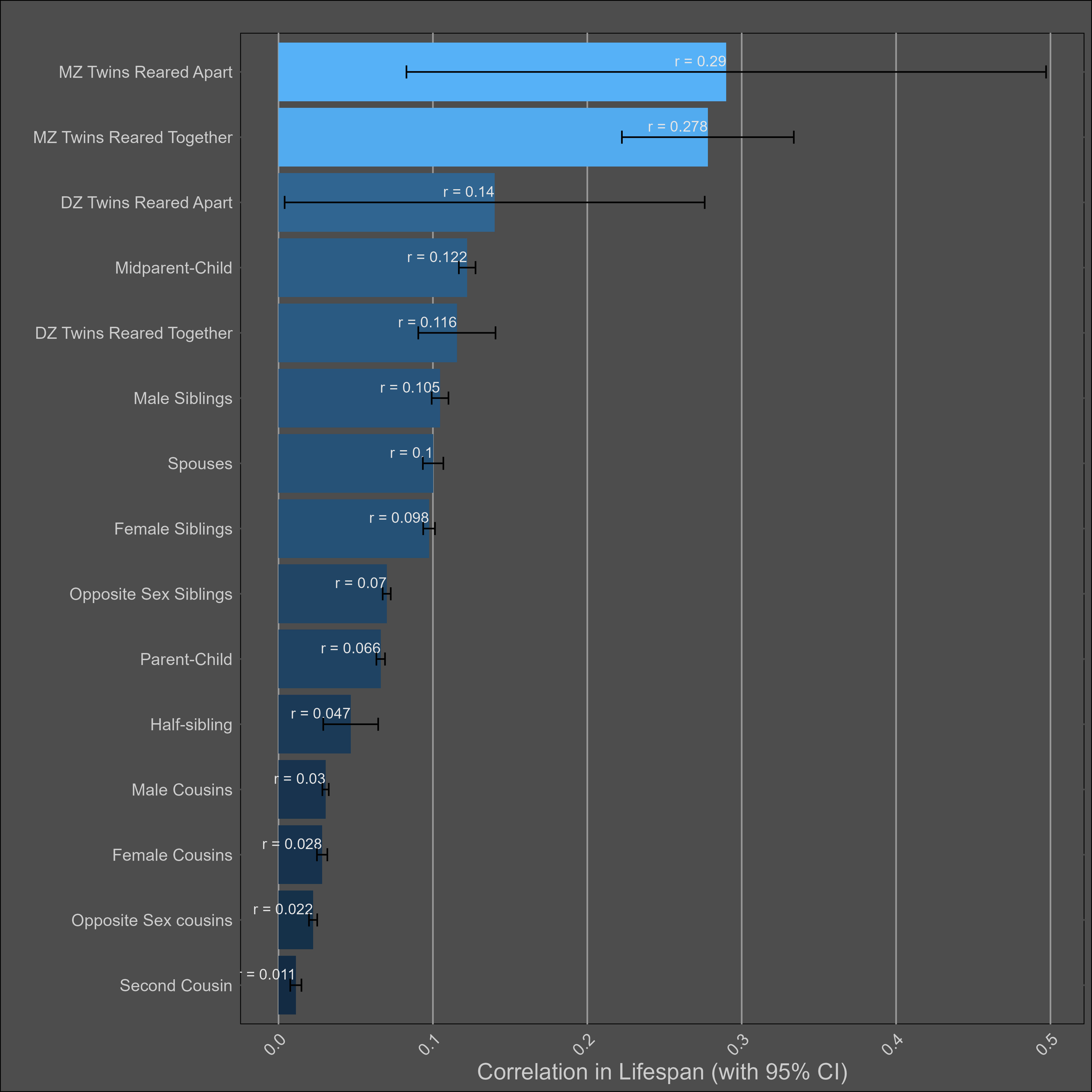
Lifespan — 20% (10%-30%)
The chart:
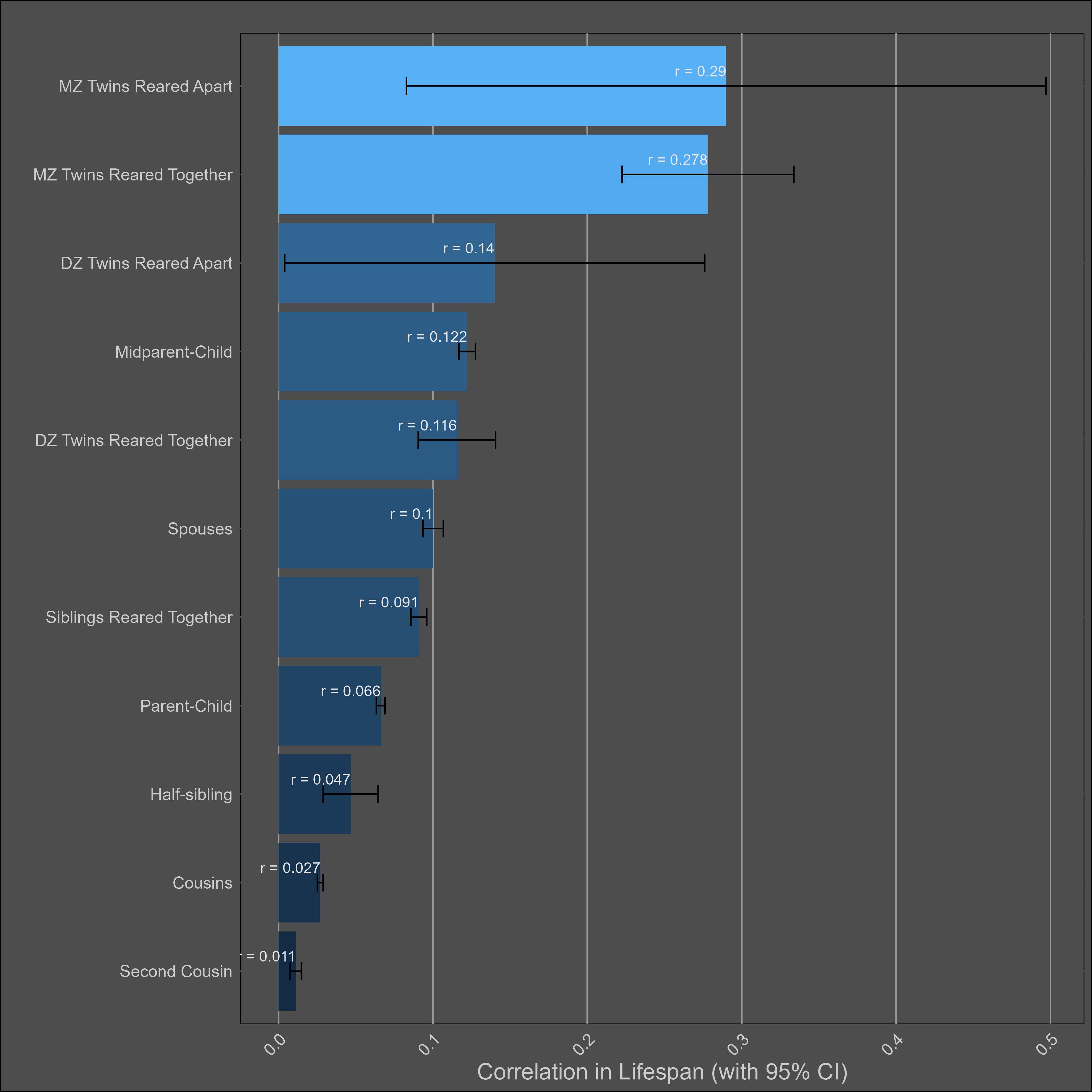
The DZ sample size is too low to test for twin-specific effects.
An ADE model fit the data best, which estimated a broad-sense heritability of 23%:
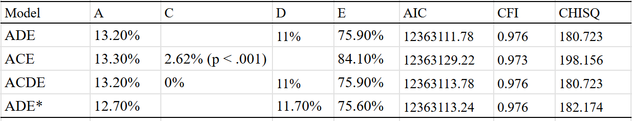
Generally I am skeptical of the idea that dominance and epistasis strongly contribute to human variation, but for the case of lifespan I think it’s possible — many monogenic disorders are recessive or dominant and have strong effects on mortality. The presence of genetic disorders that cause people to die at early ages could attenuate the effects of alleles that cause people to die less often of diseases that kill you in your old age.
Empirically, people have tried to test this hypothesis using IBD-based estimates of genetic similarity between individuals. They did find evidence for dominance, but it was weak:
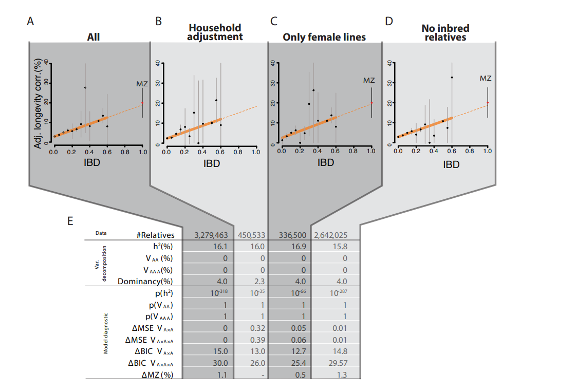
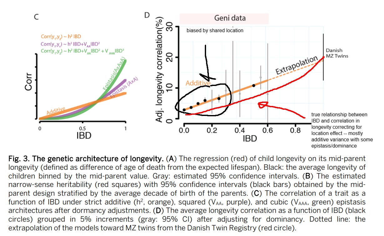
They still found little evidence for dominance, even after adjusting for household effects, but I have a different theory: that pedigree correlations are biased by location: relatives are more likely to live in the same location, and some locations have higher mortality rates than others due to non-genetic factors. Represented graphically:
The people I took the data from claim that the estimated heritability of lifespan decreases vastly upon adjusting for assortative mating. I find this extremely hard to believe. Consider that the effect of assortative mating on genotypic similarity between relatives is a function of two variables: the strength of the phenotypic assortment and the trait heritability; the higher, the larger the inflation:
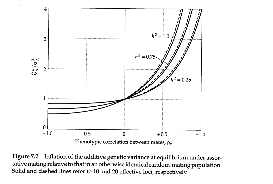
As such, there is very little reason to believe a priori that assortative mating substantially biases estimates of the heritability of lifespan. I didn’t even bother reading most of their paper, since their conclusion was so unbelievable that I thought it was worthless. No statistical model will convince me the earth is flat or that my mom is black.
Within my models, correcting for assortment only partitioned variance away from the additive component towards the dominant one.
The relatively low heritability of lifespan is due to extrinsic deaths, which occur due to infection, violence, or accidents. When these are removed, estimates of the heritability of human lifespan increase to 50-60%:
Shenhar et al 2025, Heritability of human lifespan is about 50% when confounding factors are addressed, biorxiv, doi: 10.1101/2025.04.20.649385
The heritability of human lifespan is a fundamental question in biology. Current estimates of heritability are low - twin studies show that about 20-25% of the variation in lifespan is explained by genetics, and some large family pedigree studies suggest it is as low as 7%. However, these studies do not distinguish between deaths driven by intrinsic biological processes and deaths caused by extrinsic factors such as accidents or infections. Here we use mathematical modeling and analyses of twin cohorts raised together and apart to show that extrinsic mortality skews heritability estimates by driving down measured lifespan correlations among twin pairs. We also identify a nonlinear effect of the cutoff age—the minimum age of death included in each study — on estimates of heritability. Correcting for these factors more than doubles previous estimates, revealing that intrinsic heritability of human lifespan is above 50%. Such high heritability is similar to most other complex human traits. We thus challenge the consensus that genetics has only a minor effect on lifespan and show that genes explain the majority of lifespan variation. Since genes are important, understanding the genetics of longevity can reveal aging mechanisms and inform medicine and public health.
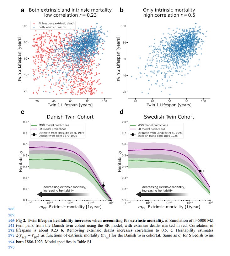
Though it would be misleading to say that, because of this, lifespan has a “true” heritability of 55% — I interpret this as biological ageing having a strong genetic component and extrinsic deaths as having a very small genetic component.
Within the last 200 years, the correlation between male relatives in lifespan has increased, while the correlation between female relatives decreased:
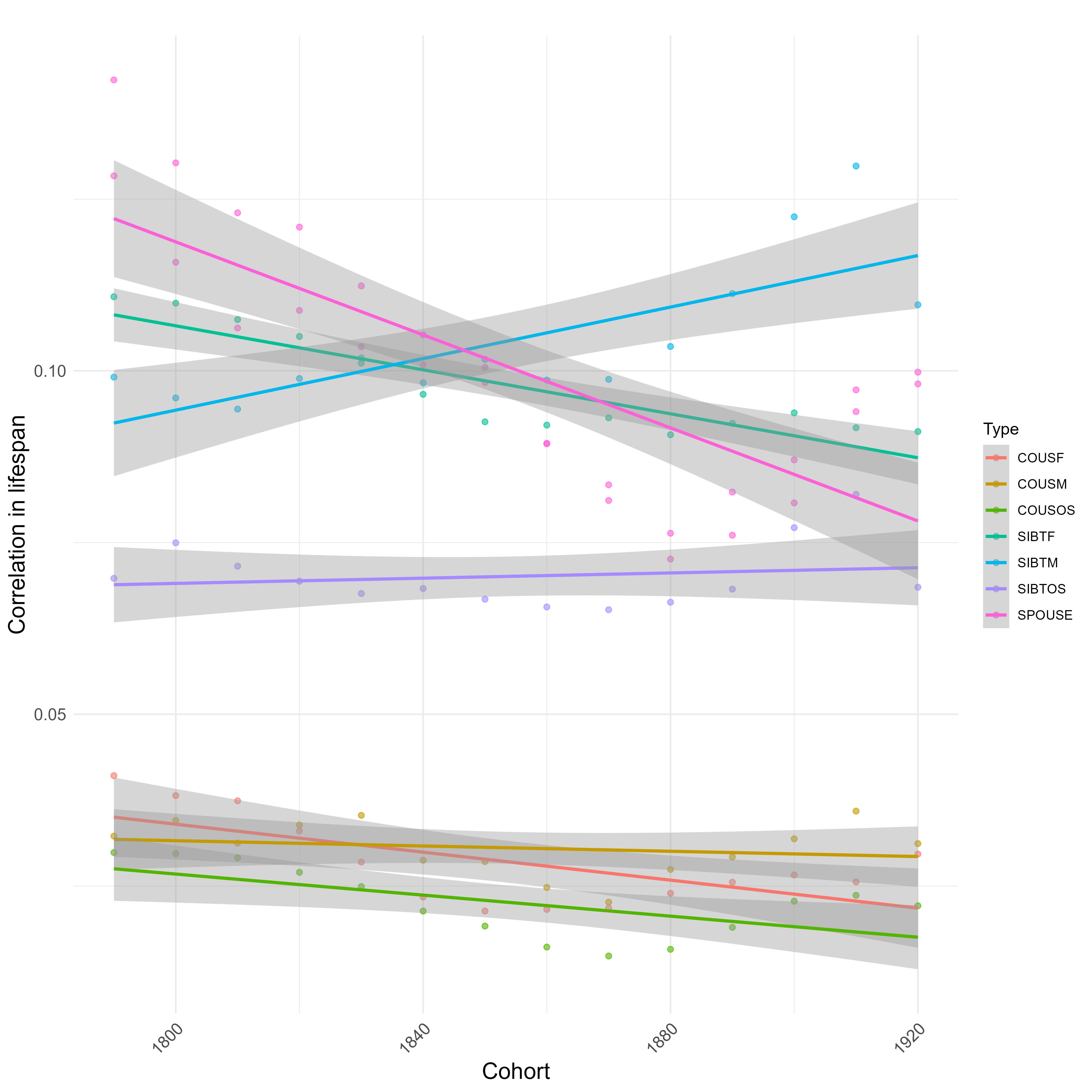
Correlations split by sex:
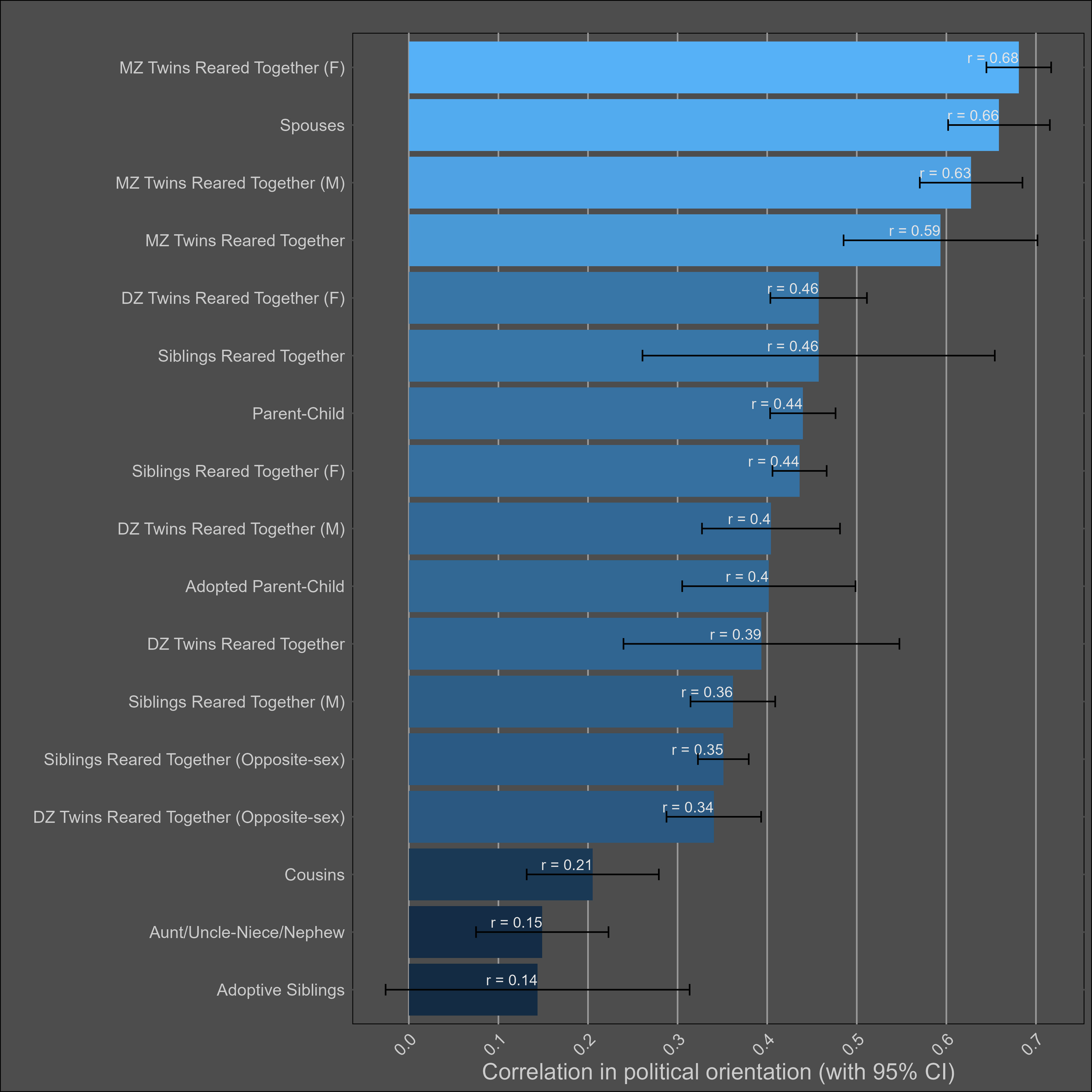
Political views — 45% (35-55%)
Most of the samples took the Wilson-Patterson scale of conservatism, which has a reliability of .94, or they self-reported their political views on a scale. I generously assumed that all scales with unknown reliabilities had an rxx of .94. I adjusted the correlations for measurement error and grouped them by type:
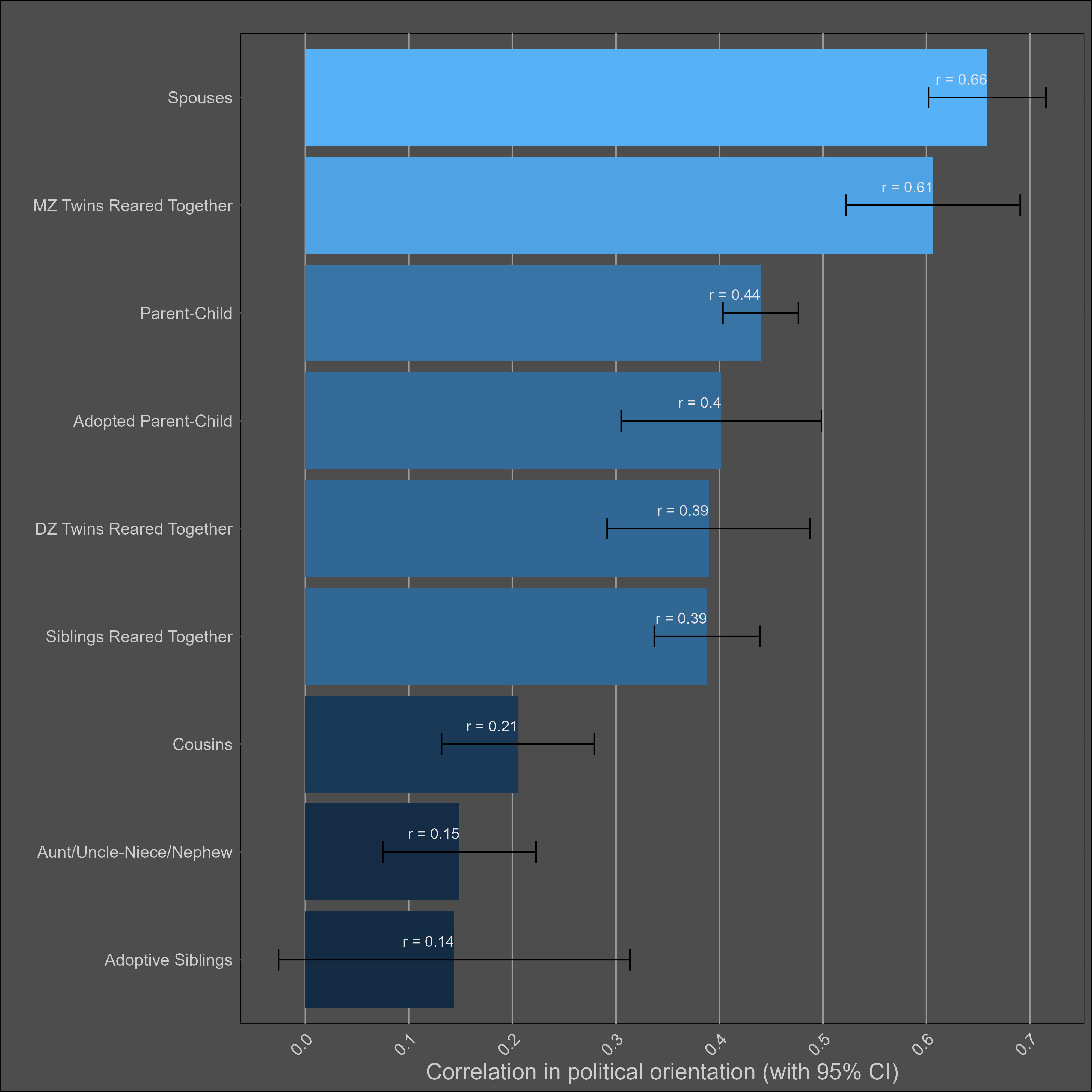
It’s clear that there are social transmission effects here; the political views of parents and their adoptive children are almost as highly correlated as those of biological parents and their children. Selective placement presumably has some role in this, but correlations between adoptive and biological parents are typically in the 0.2 - 0.4 range — not high enough to justify this correlation. Cousins are also more similar to each other in comparison to avunclars, which violates a genetic model, or implies large differences between cohorts in the effects of genes.
ACE produced non-sensical results (heritability of 69% + unshared environmental component of 30%), so I decided to try something more avant garde. A model which includes a social transmission component, where relatives have the following similarities19:
Parents and children: similarity of 1
Siblings/twins: 0.5
Cousins: similarity of 0.25
Avunclar relationships: similarity of 0.125
I then ran the ASE model, and got 47% A (additive genes), 23% S (social transmission), and 30% E (unshared environment). Not great, but it’s better than what I got with ACE. I tried a version which adjusted for assortment (p = 0.66 and h^2 = 40%), and got a heritability estimate of 40% instead.
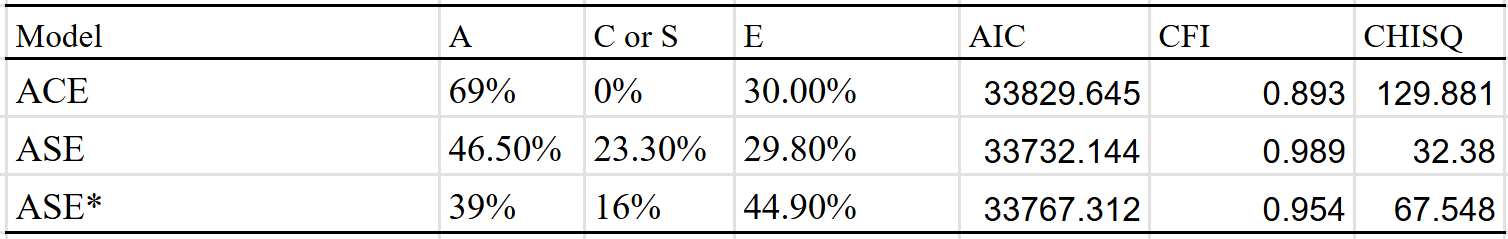
The model with the best fit is the ASE model with no adjustment, though I see no reason to think it’s the correct one, as one should expect there to be genetic consequences of assortative mating for political views. However, these corrections assume that the assortment has been occuring for multiple generations, and it’s likely that this assumption is violated.
Correlations between female family members were slightly larger than those between male family members, which in turn were larger than the opposite-sex correlations.
Getting married — 20% (10-30%)
The correlations:
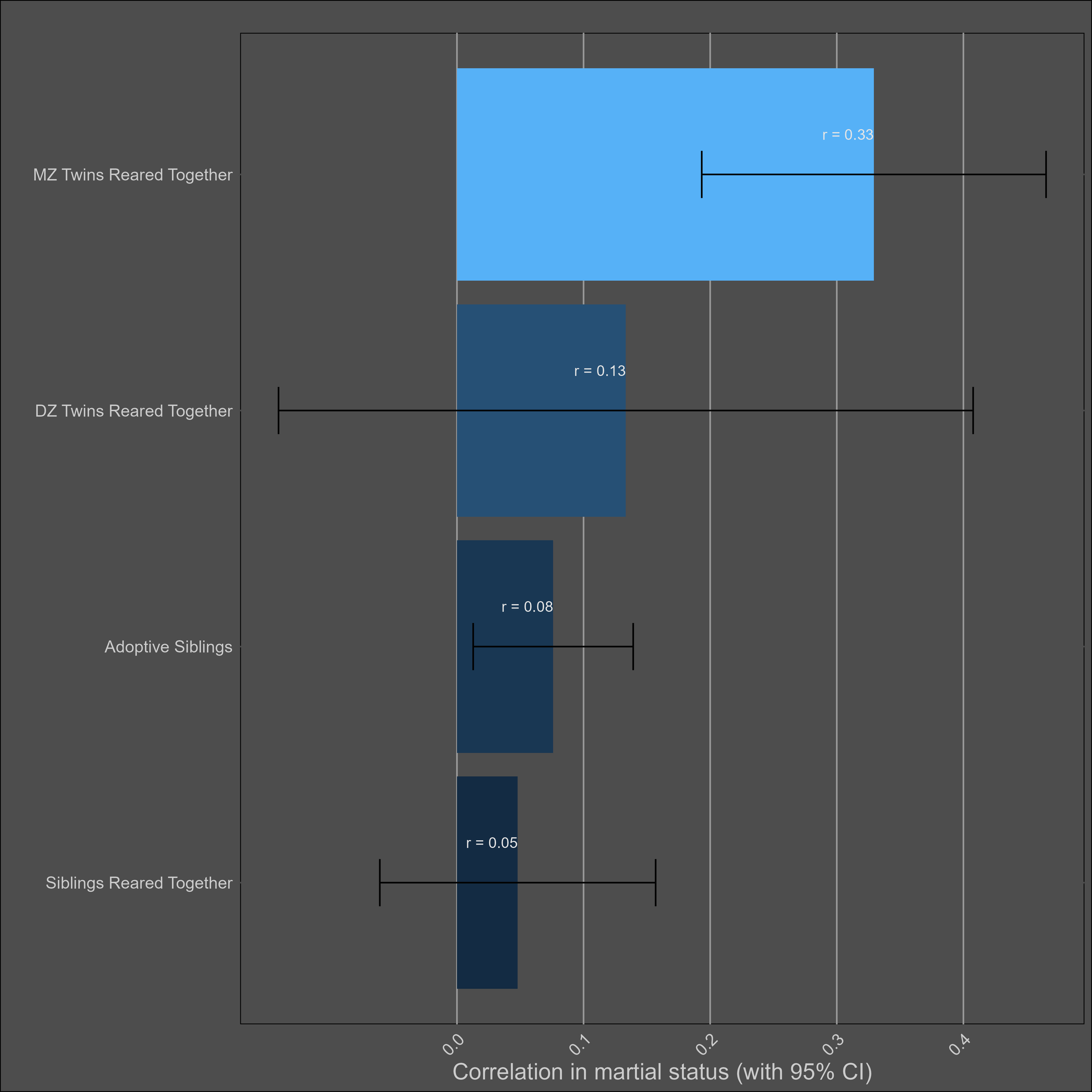
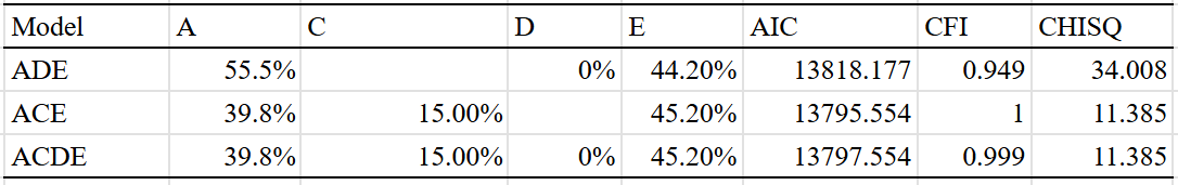
Ugly. I did my best, fit a model that made sense (ACE), and got these parameters:
A: 19.7% (95% CI = 13% - 27%)
C: 6% (95% CI = 3.2% - 9.7%)
E: 78% (95% CI = 71.9% - 84.3%)
Bizarrely enough, the variance components don’t even add up to 100%.
BMI — 55% (40% - 70%)
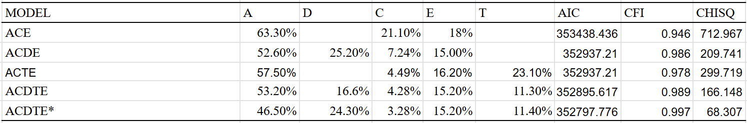
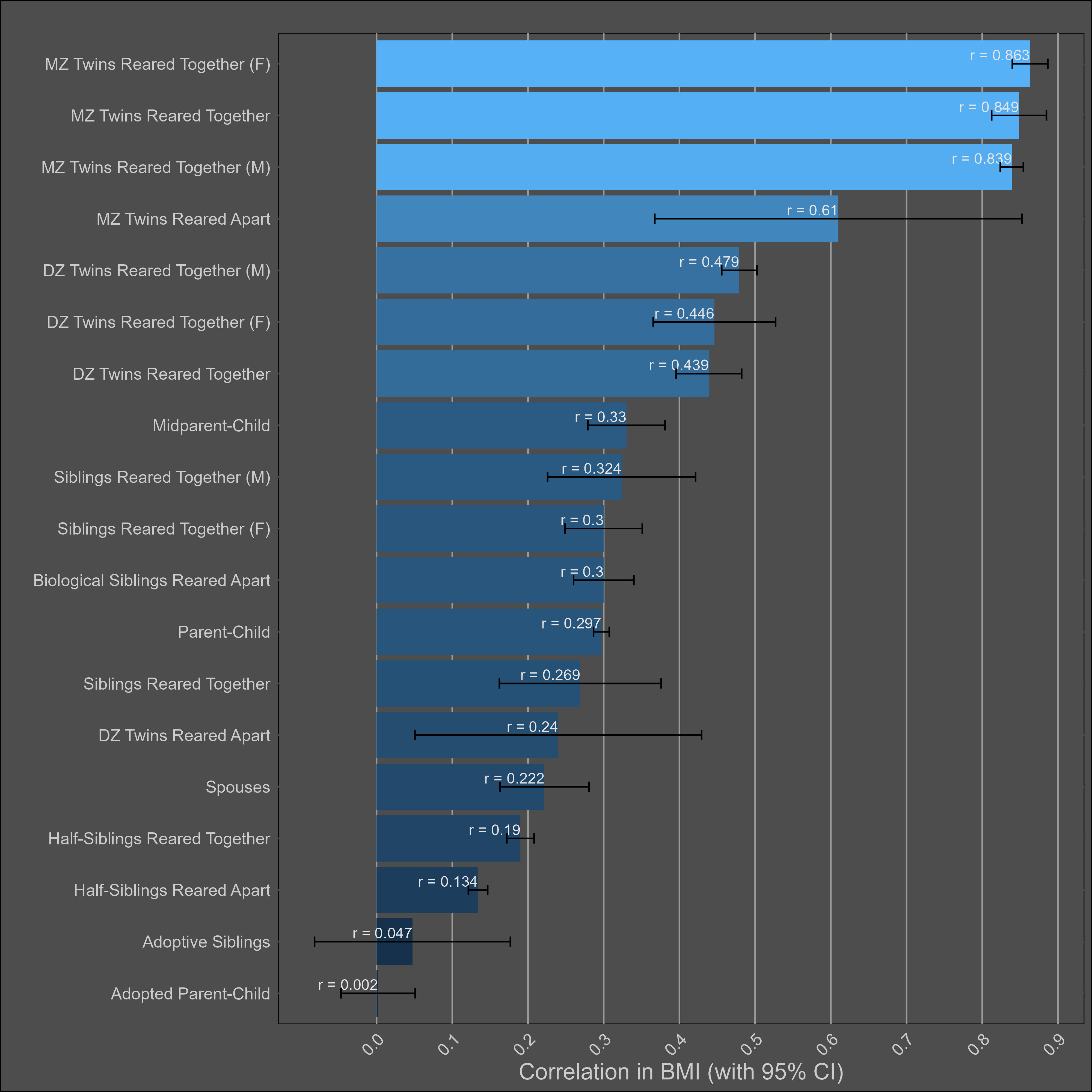
The table:
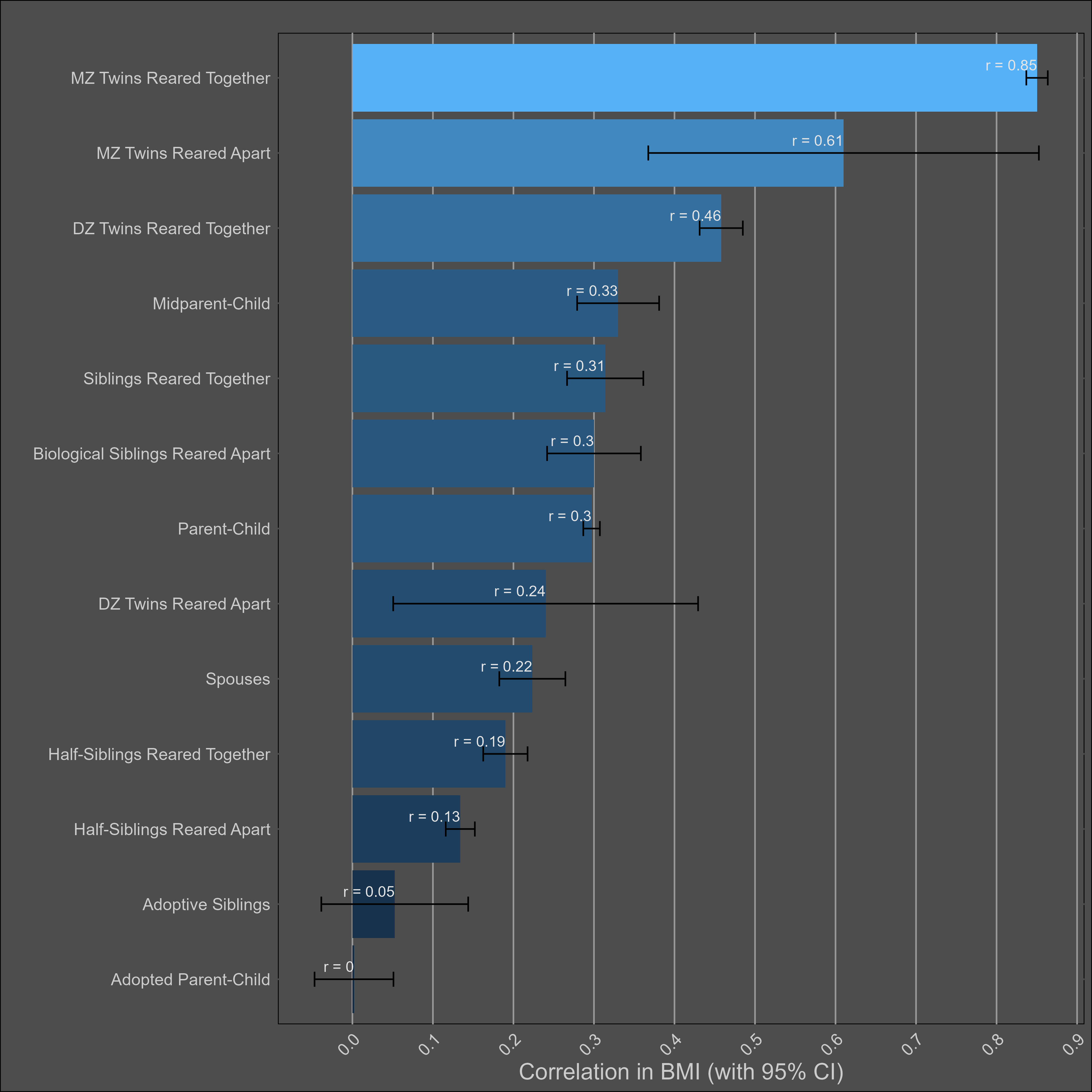
Very large twin-specific effect here — DZ twins correlate at 0.46 and siblings correlate at 0.3. Twins reared apart are less similar than those reared together, though this is hardly the case for other kin pairs. In the American adoption study of Korean children, there was no correlation between adopted parents and children, and a correlation of .11 (n = ~900 pairs) in genetically unrelated adult siblings.
Twin models give a much higher heritability estimation than a pedigree model that excludes twins reared together:
The twin model is probably wrong here, unless either epistasis or dominance is a large factor in determining how overweight people are. Personally, I suspect the problem is that the EEA assumption is violated, though I am open to being wrong — the confidence interval I assign to the heritability of BMI reflects this.
Elk’s meta-analysis of heritability estimates for BMI also found the same thing:
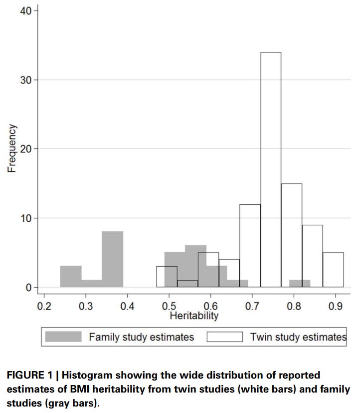
I also ran other models, which hint at the existence of a twin-specific effect. The dominant variance is also extremely large in the models that include it:
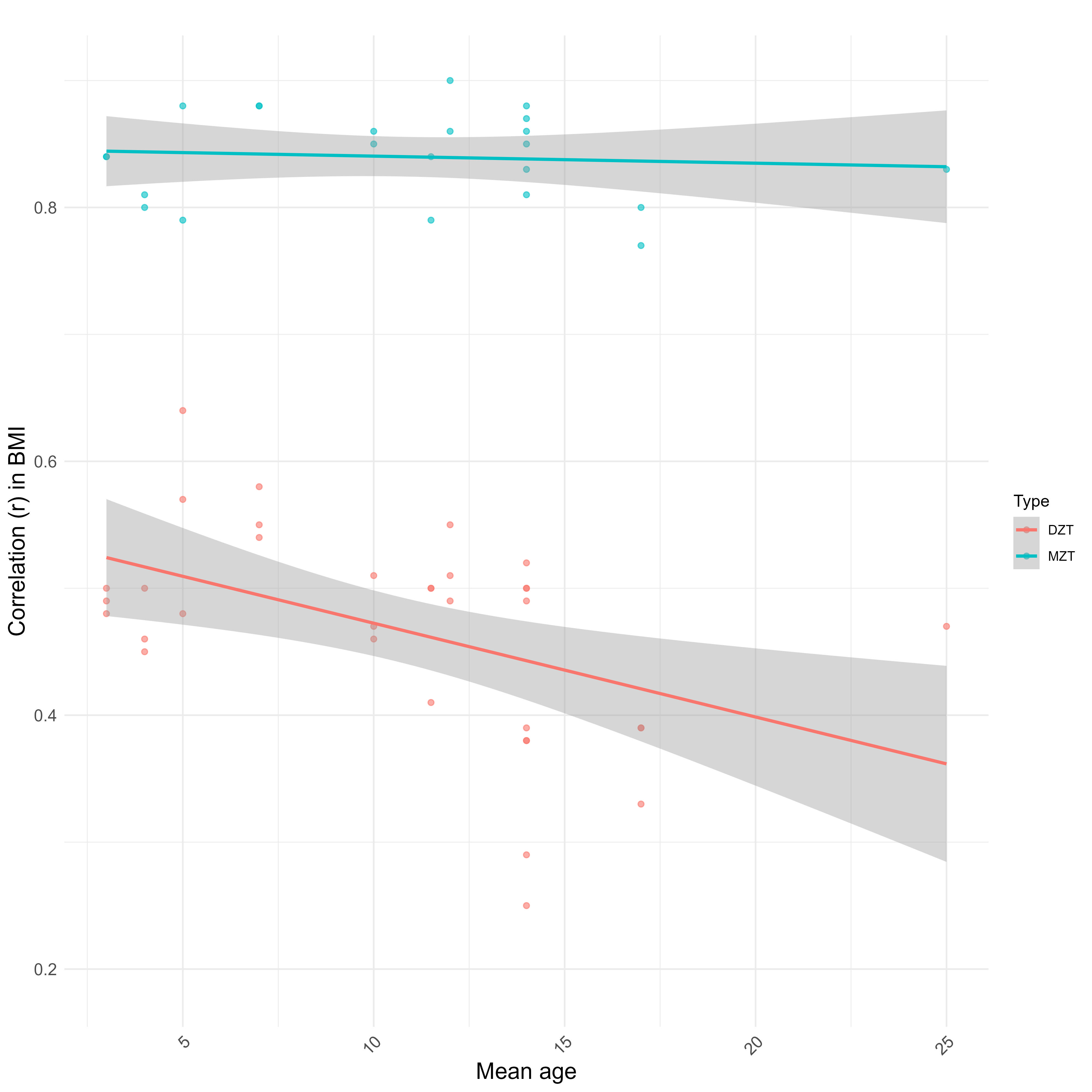
The low shared environmental component for BMI is counterintuitive, but note that most twin and family studies are often conducted in the same nation and at the same time; they will not reliably capture environmental effects that vary by location and especially by time.
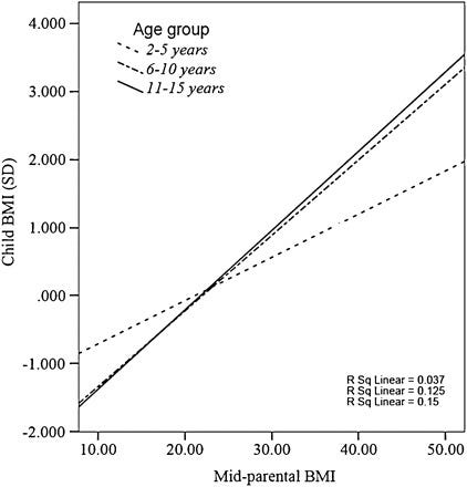
The midparent ~ child correlation (0.33) is lower in comparison to what would be expected from a heritability of 55%, but I suspect this is due to the genetic causes of BMI varying by generation and the sample in question being young; the correlation was closer to ~.4 in older children:
The Wilson effect can also be observed between studies:
Correlations split by sex:
Wealth — 30% (20% - 40%)
I assumed the reliability of self-reports of wealth was the same as those of income (0.85), adjusted the correlations accordingly, and paried them by type:
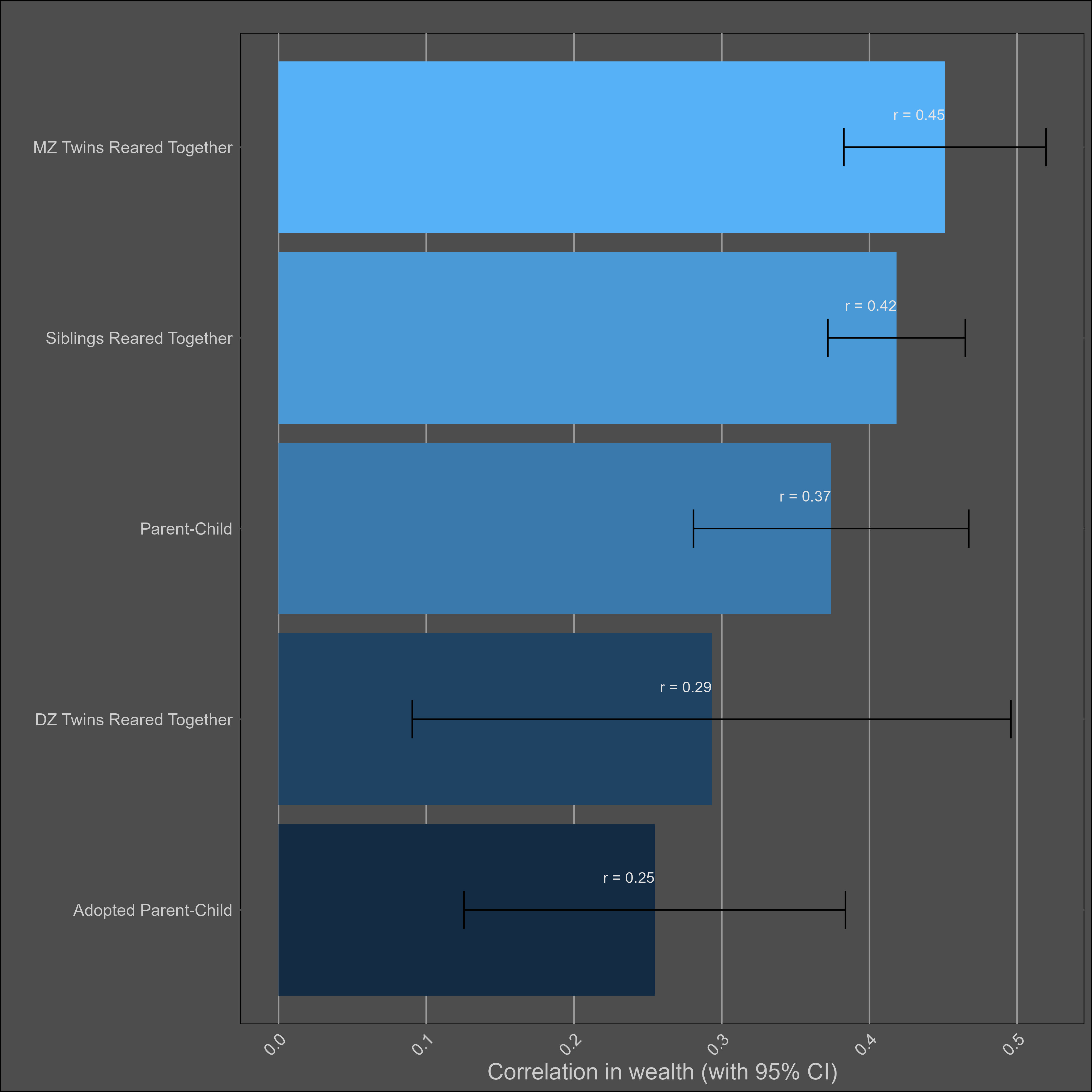
These correlations are misleading, and I was tricked the first time I saw them. Although the correlation between parents and biological children (0.37) is not much higher than the one between parents and adoptive children (0.25), statistical modelling would still imply that genetics matter more than direct phenotypic transmission. This is because the adoptive correlation has to be squared to be turned into a variance component. Therefore, this chart would imply a direct phenotypic transmission estimate of 6.2% (√0.25) and a heritability of 24% (2x(0.37-0.25)). The standard twin method estimates a similar heritability — 32% (2x(0.45-0.29).
I’m reticent to give a low heritability estimate for wealth, as income is substantially heritable and financial decisions are as well. If the heritability is generously assumed to be 30%, that implies a shared environmental effect of 14% (based on DZ twins) to 27% (based on siblings). Although no twin-specific effect is observed, it certainly exists in real life, as twin-specific effects exist for income and education.
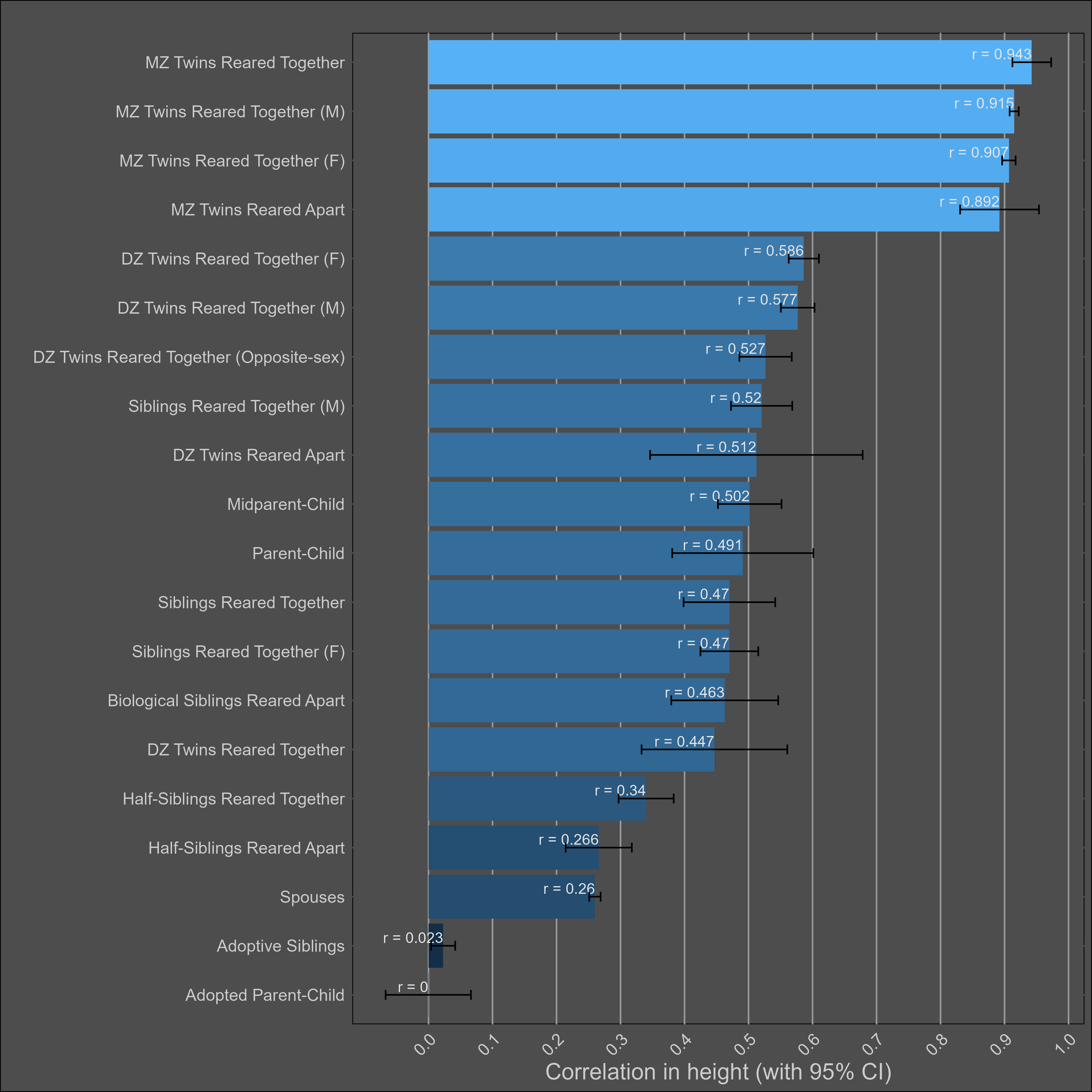
Height — 85% (80% - 90%)
The heritability of height is uncontroversially high. The kin correlations reflect this:
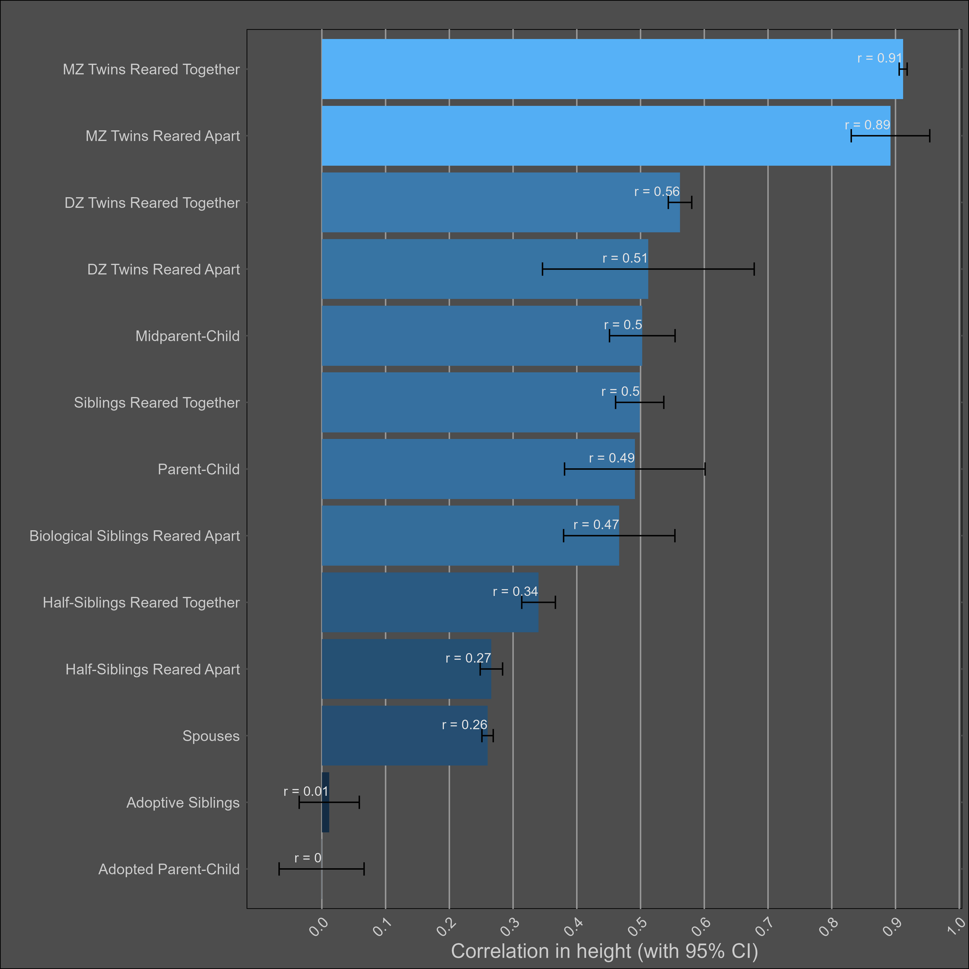
There’s a Wilson effect, where the correlation between DZ twins drops from 0.65 to 0.5 in adult samples:
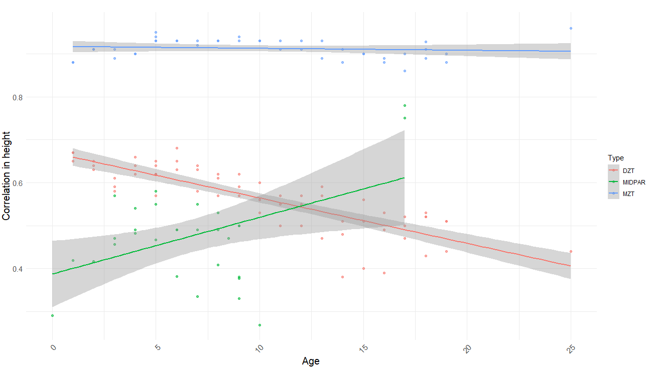
As the effect was so large, I restricted the analysis to samples with an average age of above 16. I tried four different models and got these results:
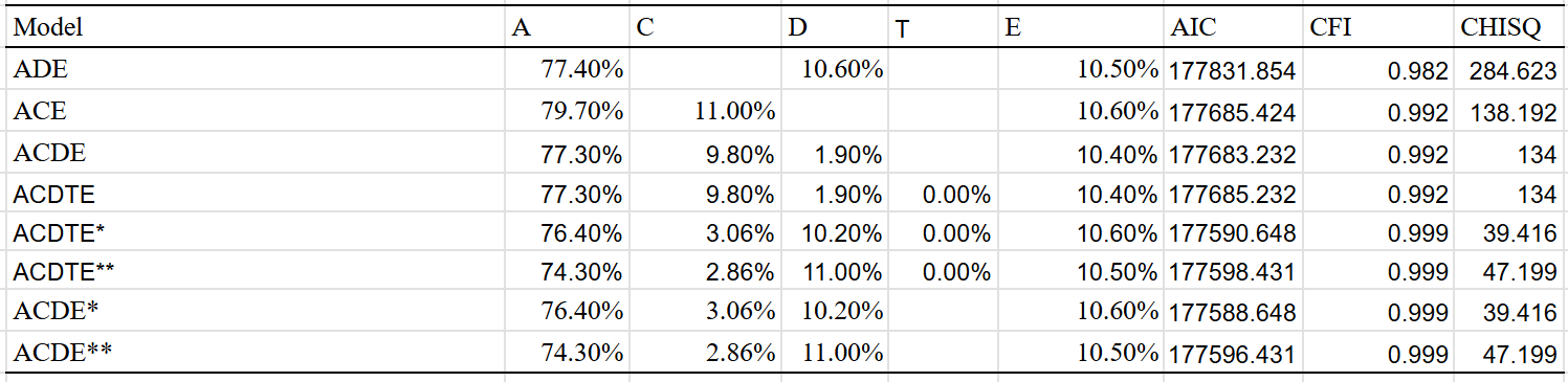
Best fit is the ACDE model that adjusted for assortment. Dominant variance was small, indicating that the results were trustable. The twin-specific effect is estimated to be zero, but I suspect that it exists to a minimal extent, even within adults.
Correlations split by sex:
Income — 40% for one year, 50% for permanent income
These are the averages by family pair for yearly income, adjusted for the reliability of self-reported income (assumed to be .85):
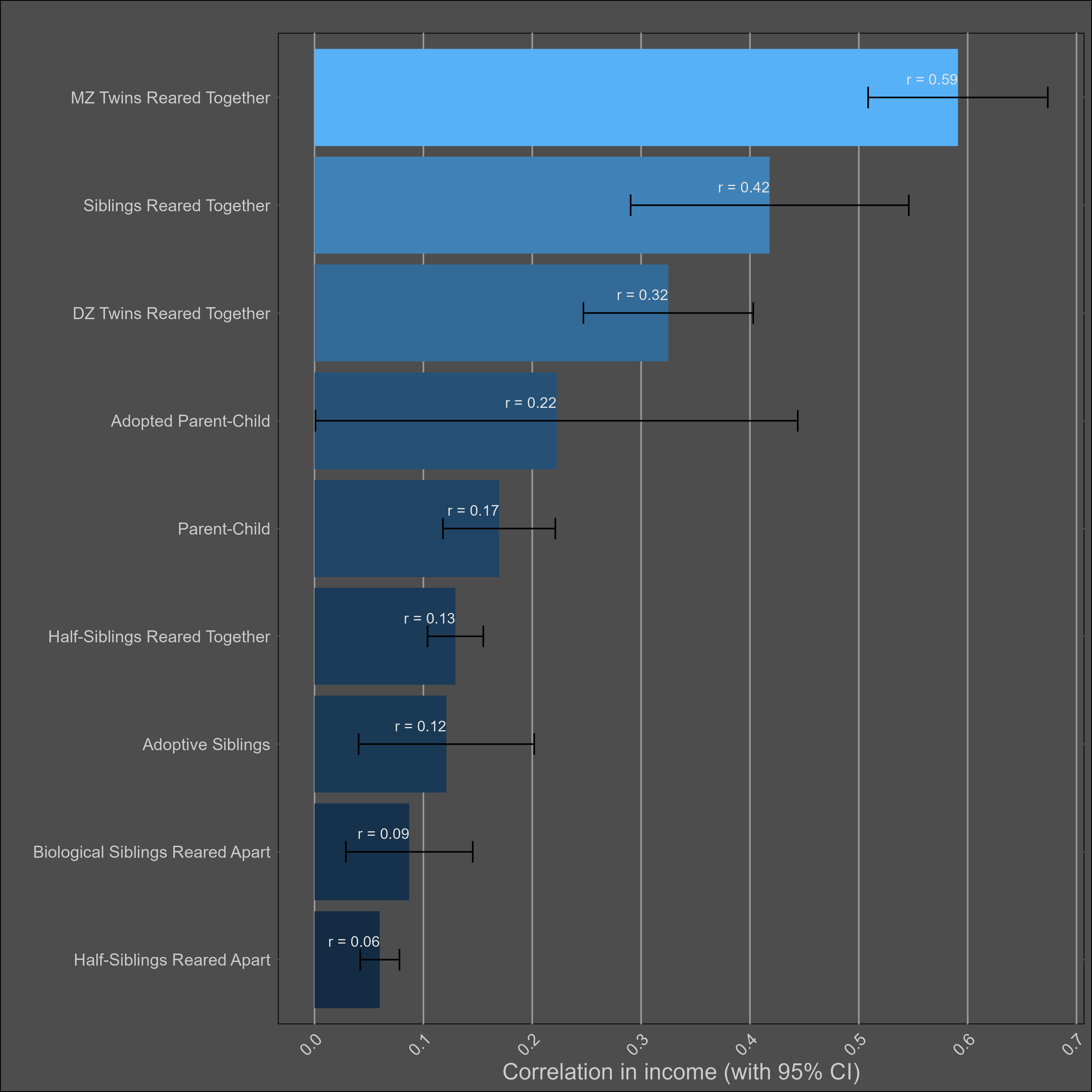
Family correlations in income are typically stronger in the United States, which I suspect is due to greater assortative mating and regional/ethnic diversity.
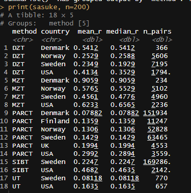
As such, the meta-analysis of correlations between family members is quite misleading. In Sweden, for example, the twin-specific effect for income (and education, for that matter) is clear, despite the meta-analysis not finding them:
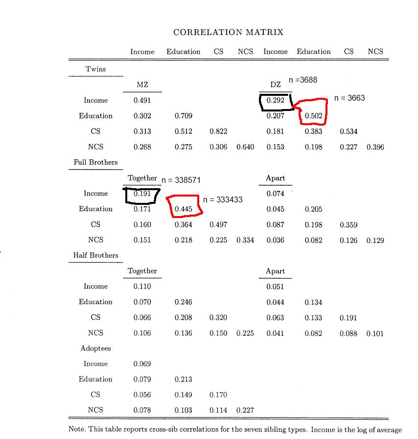
Due to this problem, I did two rounds of formal modeling; one for European countries, and another for the United States.
I’ll start with America. The correlation between adoptive parents was too imprecise to do anything interesting with, so I removed it from the data, and fit three models to the remaining 5 correlations:
ACE was the winner here, and estimated a heritability of 40% for income.
These were the results for Europe, using the same sets of family members that I used for America:
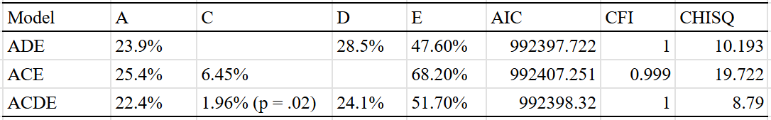
I believe these models are wrong; based on the correlations between half siblings and siblings reared apart, I suspect the true parameters for Europe are H^2 = 30-40%, C^2 = 5-10%, and E^2 = 50-60%. Rather than get hung up on the modeling, I decided to estimate the heritability of permanent income instead.
Sibling correlations in income are larger when averaged over a multi-year period, as variance in income that occurs due to time is reduced:
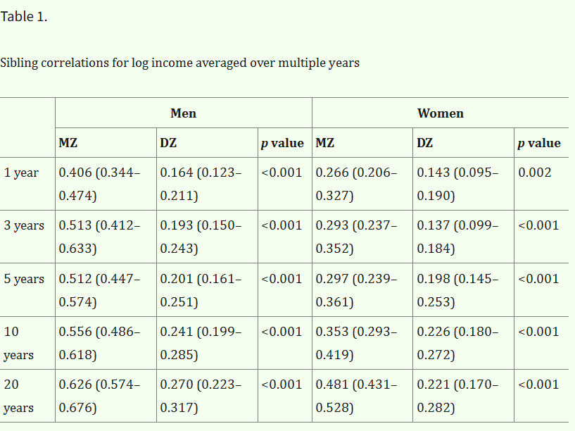
Solon noticed this in 1992 when estimating the inter-generational persistence of income, so I think the same corrections could be made for the correlations between other family pairs as well.
Rather than use the data in the prior table (which is based on Sweden), I will instead use American data to estimate the necessary correction. In the NLSY, the average year of income loads at .76 on the general factor of income, which can be used to estimate how reliable income from one year is at estimating permanent income. I then corrected the income correlations for that attenuation and reran the models:
In the best model, permanent income has a heritability of 50% and environmentality of 50%. Without using the weird correction method, Cesarini estimated a heritability of ~33% for single year income and ~52% for permanent income:
In these data, applying the simple double-the-difference estimator (Equation 7) typically produces a negative estimate of the family environment.9 We therefore instead proceed by imposing the restriction that the family environment component is zero and obtain a rough estimate of heritability by taking the average of the MZ correlation and twice the DZ correlation. This estimator suggests that heritability increases from 0.37 to 0.58 in men as we move from single-year income to a 20-year average. The corresponding figures for women are 0.28 and 0.46. These findings suggest that permanent income is more heritable than single-year income. This conclusion partly seems to reflect the fact that measurement error and transitory shocks generate a downward bias in estimates of heritability (Solon 1992, Zimmerman 1992, Mazumder 2005), consistent with our earlier conjecture that the heritability estimates of many other economic outcomes are downward biased.
Personality — 75% (60 - 90%)
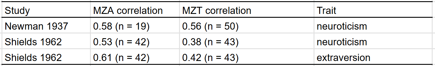
In either the Shields or Newman analysis of twins reared apart, they did find some effects of family environment on personality — twins raised by older parents were more introverted in stable and twins raised in higher SES homes were less neurotic. Despite those findings, in aggregate, the correlation in personality between MZT is about the same as that between MZA:
Most studies on the heritability of personality use self-reports, but there are two that use composites of peer and self reports20:
Riemann, R., Angleitner, A., & Strelau, J. (1997). Genetic and Environmental Influences on Personality: A Study of Twins Reared Together Using the Self- and Peer Report NEO-FFI Scales. Journal of Personality, 65(3), 449–475. doi:10.1111/j.1467-6494.1997.tb00324.x
Measured personality constructs via self- and peer reports on the items of the NEO Five-Factor Inventory. The sample included 660 monozygotic and 200 same sex and 104 opposite sex dizygotic twin pairs. Participants were aged 14–80 yrs. Self- and 2 independent peer reports for each of the twins were collected. Analysis of self-report data replicates earlier findings of a substantial genetic influence on the Big Five. This influence was also found for peer reports. Results validate findings based solely on self-reports. However, estimates of genetic contributions to phenotypic variance were substantially higher when based on peer reports or self- and peer reports because these data allowed for the separation of error variance from variance due to nonshared environmental influences. Correlations between self- and peer reports reflected the same genetic influences to a much higher extent than identical environmental effects.
Riemann, R., & Kandler, C. (2010). Construct validation using multitrait-multimethod-twin data: The case of a general factor of personality. European Journal of Personality, 24(3), 258–277. doi:10.1002/per.760
We describe a behavioural genetic extension of the classic multitrait-multimethod study design that allows estimating genetic and environmental influences on method effects in twin studies (MTMM-T). Genetic effects and effects of the environment shared by siblings are interpreted as indicators of convergent validity. In an application of the MTMM study design, we used self- and peer report data to examine the higher-order structure of the NEO-PI-R. Structural equation modelling did not support a general factor of personality in multimethod data. The higher-order factor Stability turns out to be, at most, a weak trait factor. Genetic effects on method factors indicate that especially self-reports but also peer reports show convergent validity between twins but not between methods. Copyright # 2010 John Wiley & Sons, Ltd
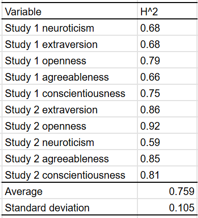
These were their main findings:
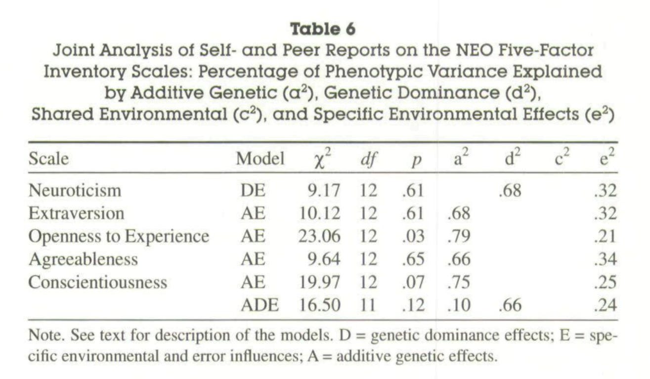
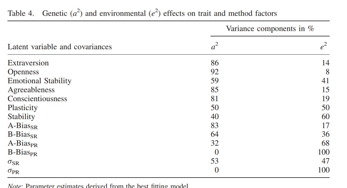
On average, the estimated heritability of a big 5 personality trait was 75% when the appropriate method was used.
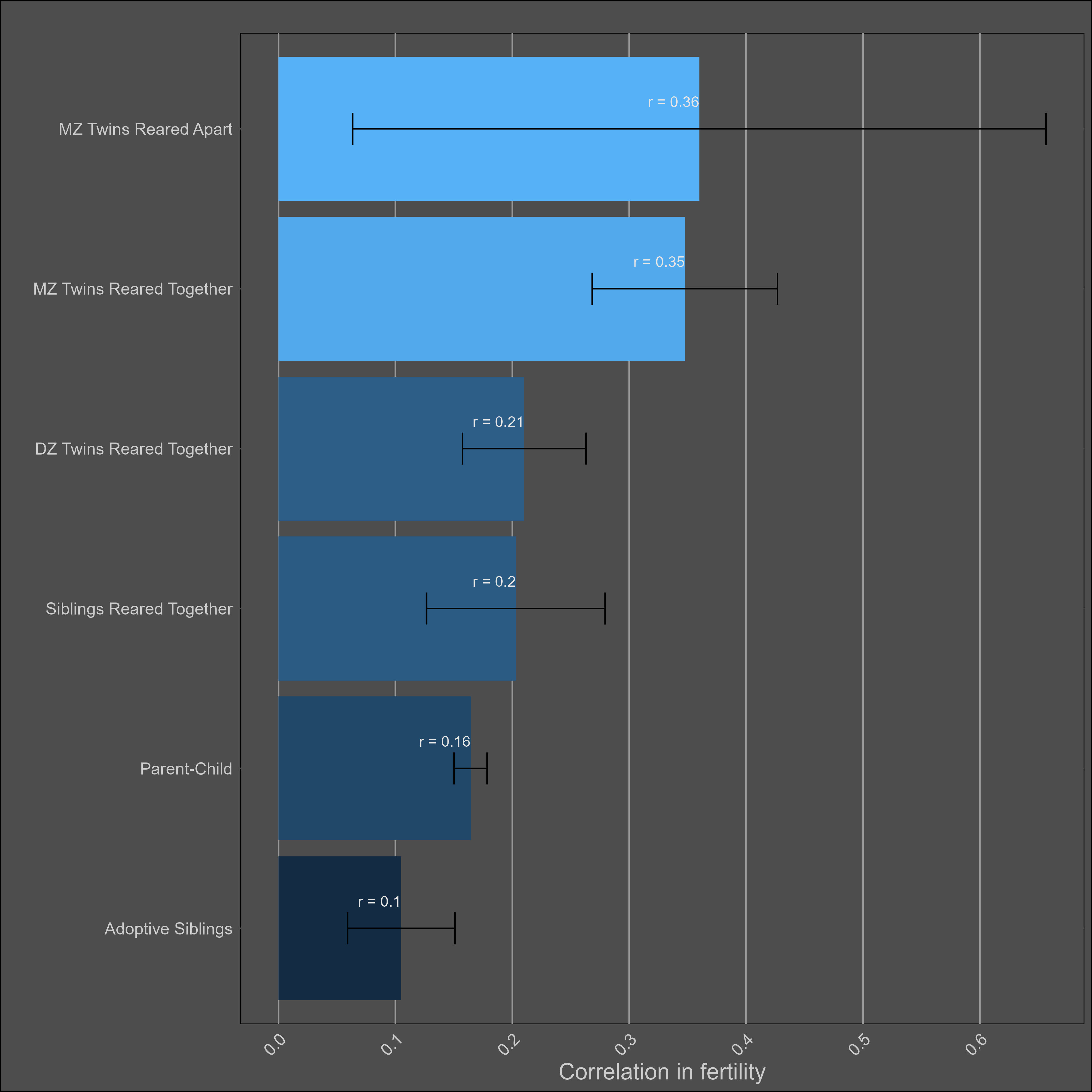
Fertility — 30% (25% - 35%)
No adjustments for reliability or misestimation were made in the calculation of averages by family pair. I restricted the data to correlations with a cohort of above 1850 or year of above 1900.
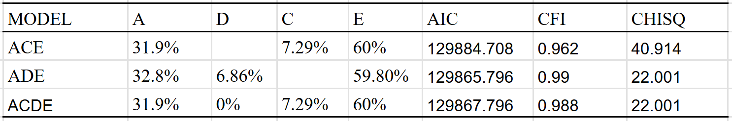
Given that there were only so many correlations, I fit these correlations to 3 simple models. The model with a shared environmental component found no evidence of dominance:
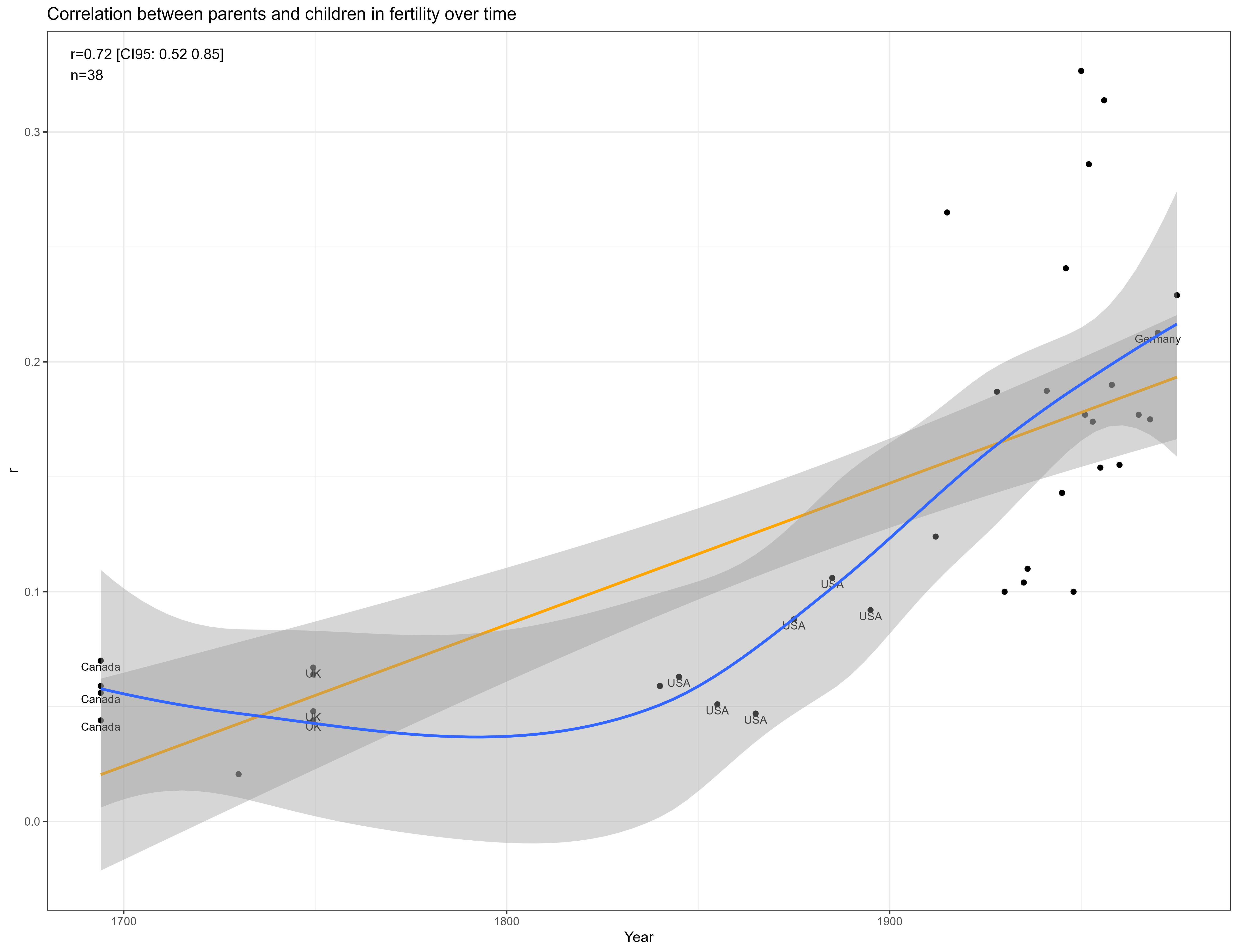
In line with prior literature, I found the correlation between parents and children in fertility has risen over time:
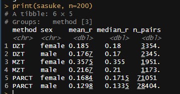
The heritability also appears to be higher in mean, with these kin correlations implying a heritability of ~35% in women and ~25% in men:
obtained through email.
I encourage plagiarism of my work.
Hard to tell exactly how much because of selective adoption and that there is only one sample of a correlation between adoptive parents and children.
Massive confidence interval.
Lifespan, intelligence, income, education, personality, BMI, height, political orientation. Admittedly, a lot of my underlying data comes from these sources.
Added Beauchamp et al to the file, revised section on education, fixed typo (MZA education correlate at .31 not .42).
EEA violations mean that the correlation between MZ twins is inflated due to environmental factors. If this is the case, then the dominance component will pick up on the surplus correlation between the MZ twins and overestimate the broad-sense heritability of the trait.
MZ twins share all epistatic interactions, while most family pairs share few of them. If epistasis occurs, then the dominance component will pick up on most of said variance, which isn’t really an issue as it’s picking up on variance that isn’t environmentally caused.
It’s possible for the effects of genetic variants to differ by generation — this has been observed to be the case for education, where there is a correlation of just .72 (se = .12) between the effects of genes between different cohorts (see page 41 of the EA3 supplement). If this is the case, then the correlation between parents and children will be lower in comparison to what would be expected from the true narrow-sense heritability. Largely a non-issue, and results in broad-sense heritability being underestimated if a dominance component (or another that has similar properties) is not added to the model.
If genes and environmental factors interact in a non-linear way, where MZ twins share most interactions while other family members share few of them, then variance caused by these interactions will be allocated to the dominance component. I actually made this up on the spot, and have no idea if non-linear interactions between genes and environments exist, but theoretically if genes and environments interact in non-linear ways, then the correlation between MZ twins will be inflated relative to other kin correlations
If any correlation exceeded 1, it was manually set to .99.
> utmeta <- metafor::rma(yi=adj_r, sei=se, data=(RMZRDz %>% filter(method=='UT')))
> summary(utmeta)

Random-Effects Model (k = 36; tau^2 estimator: REML)

  logLik  deviance       AIC       BIC      AICc
  6.5576  -13.1152   -9.1152   -6.0045   -8.7402

tau^2 (estimated amount of total heterogeneity): 0.0170 (SE = 0.0089)
tau (square root of estimated tau^2 value):      0.1303
I^2 (total heterogeneity / total variability):   56.36%
H^2 (total variability / sampling variability):  2.29

Test for Heterogeneity:
Q(df = 35) = 59.4050, p-val = 0.0062

Model Results:

estimate      se    zval    pval   ci.lb   ci.ub
  0.1874  0.0344  5.4440  <.0001  0.1199  0.2548  ***

---
Signif. codes:  0 ‘***’ 0.001 ‘**’ 0.01 ‘*’ 0.05 ‘.’ 0.1 ‘ ’ 1

>
> mztmeta <- metafor::rma(yi=adj_r, sei=se, data=(RMZRDz %>% filter(method=='MZT')))
> summary(mztmeta)

Random-Effects Model (k = 54; tau^2 estimator: REML)

  logLik  deviance       AIC       BIC      AICc
 39.3221  -78.6442  -74.6442  -70.7036  -74.4042

tau^2 (estimated amount of total heterogeneity): 0.0062 (SE = 0.0020)
tau (square root of estimated tau^2 value):      0.0787
I^2 (total heterogeneity / total variability):   81.39%
H^2 (total variability / sampling variability):  5.37

Test for Heterogeneity:
Q(df = 53) = 293.1137, p-val < .0001

Model Results:

estimate      se     zval    pval   ci.lb   ci.ub
  0.8604  0.0152  56.4397  <.0001  0.8305  0.8903  ***

---
Signif. codes:  0 ‘***’ 0.001 ‘**’ 0.01 ‘*’ 0.05 ‘.’ 0.1 ‘ ’ 1

>
> dztmeta <- metafor::rma(yi=adj_r, sei=se, data=(RMZRDz %>% filter(method=='DZT')))
> summary(dztmeta)

Random-Effects Model (k = 52; tau^2 estimator: REML)

  logLik  deviance       AIC       BIC      AICc
 17.0097  -34.0193  -30.0193  -26.1557  -29.7693

tau^2 (estimated amount of total heterogeneity): 0.0106 (SE = 0.0041)
tau (square root of estimated tau^2 value):      0.1029
I^2 (total heterogeneity / total variability):   75.96%
H^2 (total variability / sampling variability):  4.16

Test for Heterogeneity:
Q(df = 51) = 164.9586, p-val < .0001

Model Results:

estimate      se     zval    pval   ci.lb   ci.ub
  0.5672  0.0229  24.7871  <.0001  0.5224  0.6121  ***

---
Signif. codes:  0 ‘***’ 0.001 ‘**’ 0.01 ‘*’ 0.05 ‘.’ 0.1 ‘ ’ 1

>
> sibtmeta <- metafor::rma(yi=adj_r, sei=se, data=(RMZRDz %>% filter(method=='SIBT')))
> summary(sibtmeta)

Random-Effects Model (k = 64; tau^2 estimator: REML)

  logLik  deviance       AIC       BIC      AICc
 22.1491  -44.2982  -40.2982  -36.0119  -40.0982

tau^2 (estimated amount of total heterogeneity): 0.0092 (SE = 0.0033)
tau (square root of estimated tau^2 value):      0.0961
I^2 (total heterogeneity / total variability):   90.84%
H^2 (total variability / sampling variability):  10.91

Test for Heterogeneity:
Q(df = 63) = 288.2336, p-val < .0001

Model Results:

estimate      se     zval    pval   ci.lb   ci.ub
  0.5014  0.0194  25.8435  <.0001  0.4633  0.5394  ***

---
Signif. codes:  0 ‘***’ 0.001 ‘**’ 0.01 ‘*’ 0.05 ‘.’ 0.1 ‘ ’ 1

>
> mzameta <- metafor::rma(yi=adj_r, sei=se, data=(RMZRDz %>% filter(method=='MZA')))
> summary(mzameta)

Random-Effects Model (k = 10; tau^2 estimator: REML)

  logLik  deviance       AIC       BIC      AICc
  5.6736  -11.3472   -7.3472   -6.9528   -5.3472

tau^2 (estimated amount of total heterogeneity): 0 (SE = 0.0067)
tau (square root of estimated tau^2 value):      0
I^2 (total heterogeneity / total variability):   0.00%
H^2 (total variability / sampling variability):  1.00

Test for Heterogeneity:
Q(df = 9) = 2.3063, p-val = 0.9856

Model Results:

estimate      se     zval    pval   ci.lb   ci.ub
  0.7710  0.0423  18.2133  <.0001  0.6880  0.8540  ***

---
Signif. codes:  0 ‘***’ 0.001 ‘**’ 0.01 ‘*’ 0.05 ‘.’ 0.1 ‘ ’ 1

>
> sibameta <- metafor::rma(yi=adj_r, sei=se, data=(RMZRDz %>% filter(method=='SIBA')))
> summary(sibameta)

Random-Effects Model (k = 3; tau^2 estimator: REML)

  logLik  deviance       AIC       BIC      AICc
  2.4995   -4.9991   -0.9991   -3.6128   11.0009

tau^2 (estimated amount of total heterogeneity): 0 (SE = 0.0039)
tau (square root of estimated tau^2 value):      0
I^2 (total heterogeneity / total variability):   0.00%
H^2 (total variability / sampling variability):  1.00

Test for Heterogeneity:
Q(df = 2) = 1.1115, p-val = 0.5737

Model Results:

estimate      se     zval    pval   ci.lb   ci.ub
  0.3830  0.0182  21.0392  <.0001  0.3473  0.4187  ***

---
Signif. codes:  0 ‘***’ 0.001 ‘**’ 0.01 ‘*’ 0.05 ‘.’ 0.1 ‘ ’ 1

>
> hsibtmeta <- metafor::rma(yi=adj_r, sei=se, data=(RMZRDz %>% filter(method=='HSIBT')))
> summary(hsibtmeta)

Random-Effects Model (k = 9; tau^2 estimator: REML)

  logLik  deviance       AIC       BIC      AICc
  4.6602   -9.3204   -5.3204   -5.1615   -2.9204

tau^2 (estimated amount of total heterogeneity): 0.0062 (SE = 0.0050)
tau (square root of estimated tau^2 value):      0.0787
I^2 (total heterogeneity / total variability):   74.06%
H^2 (total variability / sampling variability):  3.86

Test for Heterogeneity:
Q(df = 8) = 28.6201, p-val = 0.0004

Model Results:

estimate      se     zval    pval   ci.lb   ci.ub
  0.3998  0.0342  11.6964  <.0001  0.3328  0.4668  ***

---
Signif. codes:  0 ‘***’ 0.001 ‘**’ 0.01 ‘*’ 0.05 ‘.’ 0.1 ‘ ’ 1

>
> parmeta <- metafor::rma(yi=adj_r, sei=se, data=(RMZRDz %>% filter(method=='PARCT')))
> summary(parmeta)

Random-Effects Model (k = 53; tau^2 estimator: REML)

  logLik  deviance       AIC       BIC      AICc
 27.1848  -54.3697  -50.3697  -46.4672  -50.1248

tau^2 (estimated amount of total heterogeneity): 0.0057 (SE = 0.0019)
tau (square root of estimated tau^2 value):      0.0757
I^2 (total heterogeneity / total variability):   73.21%
H^2 (total variability / sampling variability):  3.73

Test for Heterogeneity:
Q(df = 52) = 189.4809, p-val < .0001

Model Results:

estimate      se     zval    pval   ci.lb   ci.ub
  0.3794  0.0149  25.3808  <.0001  0.3501  0.4087  ***

---
Signif. codes:  0 ‘***’ 0.001 ‘**’ 0.01 ‘*’ 0.05 ‘.’ 0.1 ‘ ’ 1

>
> midparmeta <- metafor::rma(yi=adj_r, sei=se, data=(RMZRDz %>% filter(method=='MIDPAR')))
> summary(midparmeta)

Random-Effects Model (k = 10; tau^2 estimator: REML)

  logLik  deviance       AIC       BIC      AICc
 11.2564  -22.5127  -18.5127  -18.1183  -16.5127

tau^2 (estimated amount of total heterogeneity): 0.0017 (SE = 0.0020)
tau (square root of estimated tau^2 value):      0.0407
I^2 (total heterogeneity / total variability):   42.12%
H^2 (total variability / sampling variability):  1.73

Test for Heterogeneity:
Q(df = 9) = 16.2663, p-val = 0.0615

Model Results:

estimate      se     zval    pval   ci.lb   ci.ub
  0.6203  0.0213  29.1238  <.0001  0.5786  0.6620  ***

---
Signif. codes:  0 ‘***’ 0.001 ‘**’ 0.01 ‘*’ 0.05 ‘.’ 0.1 ‘ ’ 1

>
> uparmeta <- metafor::rma(yi=adj_r, sei=se, data=(RMZRDz %>% filter(method=='UPARCT')))
> summary(uparmeta)

Random-Effects Model (k = 14; tau^2 estimator: REML)

  logLik  deviance       AIC       BIC      AICc
 12.0010  -24.0020  -20.0020  -18.8721  -18.8020

tau^2 (estimated amount of total heterogeneity): 0.0026 (SE = 0.0032)
tau (square root of estimated tau^2 value):      0.0507
I^2 (total heterogeneity / total variability):   31.39%
H^2 (total variability / sampling variability):  1.46

Test for Heterogeneity:
Q(df = 13) = 17.8023, p-val = 0.1652

Model Results:

estimate      se    zval    pval   ci.lb   ci.ub
  0.1363  0.0250  5.4560  <.0001  0.0873  0.1853  ***

---
Signif. codes:  0 ‘***’ 0.001 ‘**’ 0.01 ‘*’ 0.05 ‘.’ 0.1 ‘ ’ 1

>
> metafor::regtest(x=adj_r, sei=se, data=(RMZRDz %>% filter(method=='MZT')), model='rma')

Regression Test for Funnel Plot Asymmetry

Model:     mixed-effects meta-regression model
Predictor: standard error

Test for Funnel Plot Asymmetry: z = -0.5043, p = 0.6140
Limit Estimate (as sei -> 0):   b =  0.8680 (CI: 0.8259, 0.9101)

> metafor::regtest(x=adj_r, sei=se, data=(RMZRDz %>% filter(method=='DZT')), model='rma')

Regression Test for Funnel Plot Asymmetry

Model:     mixed-effects meta-regression model
Predictor: standard error

Test for Funnel Plot Asymmetry: z = 0.7400, p = 0.4593
Limit Estimate (as sei -> 0):   b = 0.5512 (CI: 0.4894, 0.6130)

> metafor::regtest(x=adj_r, sei=se, data=(RMZRDz %>% filter(method=='SIBT')), model='rma')

Regression Test for Funnel Plot Asymmetry

Model:     mixed-effects meta-regression model
Predictor: standard error

Test for Funnel Plot Asymmetry: z = -1.3756, p = 0.1690
Limit Estimate (as sei -> 0):   b =  0.5258 (CI: 0.4757, 0.5759)

> metafor::regtest(x=adj_r, sei=se, data=(RMZRDz %>% filter(method=='MZA')), model='rma')

Regression Test for Funnel Plot Asymmetry

Model:     mixed-effects meta-regression model
Predictor: standard error

Test for Funnel Plot Asymmetry: z = -0.2664, p = 0.7899
Limit Estimate (as sei -> 0):   b =  0.7912 (CI: 0.6213, 0.9610)

> metafor::regtest(x=adj_r, sei=se, data=(RMZRDz %>% filter(method=='SIBA')), model='rma')

Regression Test for Funnel Plot Asymmetry

Model:     mixed-effects meta-regression model
Predictor: standard error

Test for Funnel Plot Asymmetry: z = 1.0410, p = 0.2979
Limit Estimate (as sei -> 0):   b = 0.3608 (CI: 0.3058, 0.4157)

> metafor::regtest(x=adj_r, sei=se, data=(RMZRDz %>% filter(method=='HSIBT')), model='rma')

Regression Test for Funnel Plot Asymmetry

Model:     mixed-effects meta-regression model
Predictor: standard error

Test for Funnel Plot Asymmetry: z = -0.4865, p = 0.6266
Limit Estimate (as sei -> 0):   b =  0.4357 (CI: 0.2673, 0.6042)

> metafor::regtest(x=adj_r, sei=se, data=(RMZRDz %>% filter(method=='PARCT')), model='rma')

Regression Test for Funnel Plot Asymmetry

Model:     mixed-effects meta-regression model
Predictor: standard error

Test for Funnel Plot Asymmetry: z = -0.7480, p = 0.4545
Limit Estimate (as sei -> 0):   b =  0.3902 (CI: 0.3496, 0.4308)

> metafor::regtest(x=adj_r, sei=se, data=(RMZRDz %>% filter(method=='MIDPAR')), model='rma')

Regression Test for Funnel Plot Asymmetry

Model:     mixed-effects meta-regression model
Predictor: standard error

Test for Funnel Plot Asymmetry: z = -0.3003, p = 0.7640
Limit Estimate (as sei -> 0): b = 0.6353 (CI: 0.5328, 0.7377)Fits:
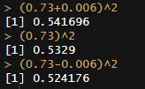
R output:
0.15^2 = 0.02, and then x2 for each parent. Slightly overestimated due to the presence of assortative mating.
Subtracting the adoptive correlation from the biological correlation yields the correlation that would be observed in the event of only genetic tranmission. In this case, it is 0.31 (0.4-0.09). A phenotypic correlation between spouses of 0.6 suggests that the coefficient for additive genetic variance for the parent~child correlation is 0.8 ( 1/2 x (1+0.6) = 0.8). Dividing 0.31 by 0.8 yields a narrow sense heritability estimate of 0.39 — 39%. Not making this correction would lead to an estimate of 50%.
Initially my brain assumed green = genes here and switched the A and E components.
All of these numbers are made up.
h/t Emil Kirkegaard
Great analysis!
This is impressive work! I'm very pleased with the contributions you've made to the behavioral knowledge on this one.
My notes:
"It’s a myth that C^2 = 0 in adults; Cesarini found that scores of genetically unrelated siblings on the Swedish military entrance exam, taken at the age of about 18, correlate at .17 (n = 1,647 individuals). We also have not found any trait with a shared environmental effect of zero that has a heritability of below 100%, so our priors for this being the one are, well, low."
Thanks to my time researching this matter, I'm immediately suspicious of shared environment values significantly different from zero for most traits other than education or wealth. You state that you control for age, but how old are we talking? The Wilson effect appears to continue well into adulthood and I'm curious how the C effect behaves with age with many of these.
"Twin models give a much higher heritability estimation than a pedigree model that excludes twins reared together:
The twin model is probably wrong here, unless either epistasis or dominance is a large factor in determining how overweight people are. Personally, I suspect the problem is that the EEA assumption is violated"
Why can't non-additive heredity be involved with BMI here? It does appear that non-additive heredity is important on the population level (and this may be behind the low heritabilities found by molecular genetic studies). Although numerically it does look like you have a fit to a violated EEA.
With income, your method doesn't allow for teasing out the sources that could inflate C (assortative mating, the Wilson effect), so it's unclear if a C significantly different from zero is real.
"Most of the samples took the Wilson-Patterson scale of conservatism, which has a reliability of .94, or they self-reported their political views on a scale."
For political views, the fraction self-reporting their political views may be a significant factor. A "conservative" in New York means something different from a "conservative" in Texas. Any way to disaggregate this from the data?
"It’s clear that there are social transmission effects here; the political views of parents and their adoptive children are almost as highly correlated as those of biological parents and their children."
There is a cohort effect on political views. I suspect that your point about environmental confounding could very well be at play. It's suspicious that adoptive parent-child correlations are so much higher than adoptive sib correlations.
Once again, great work!