Checking the Numbers: did homicide rates in England decline due to the death penalty?

No

Jul 03, 2024

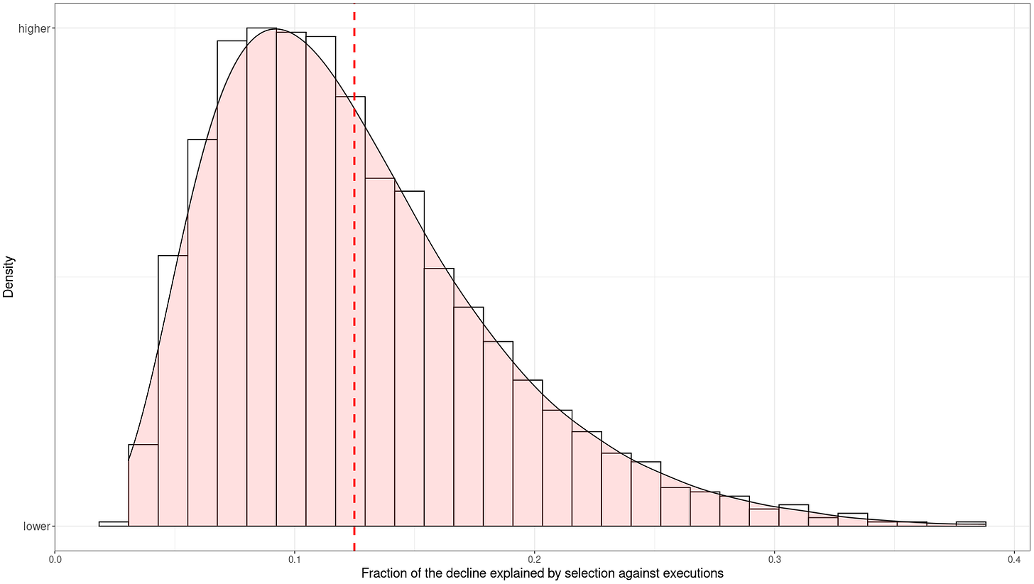
TL;DR: selection against being executed can explain roughly 11.4% (95% credible interval: [5.2%, 23.4%]) of the decline in homicide rates in England that occurred between 1300 and 1700.

______________________________

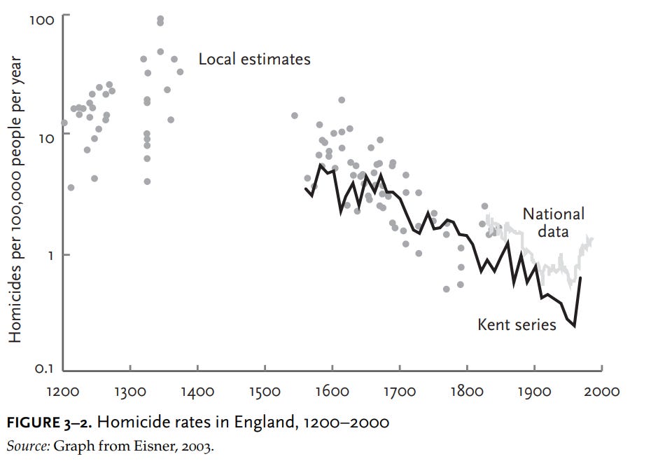
Statisticians and historians, such as Steven Pinker, have noted that homicide rates have declined in England since the Medieval period:

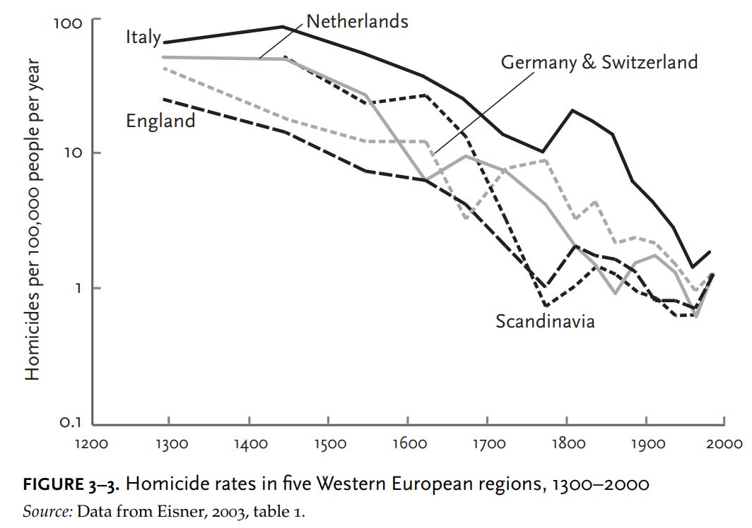
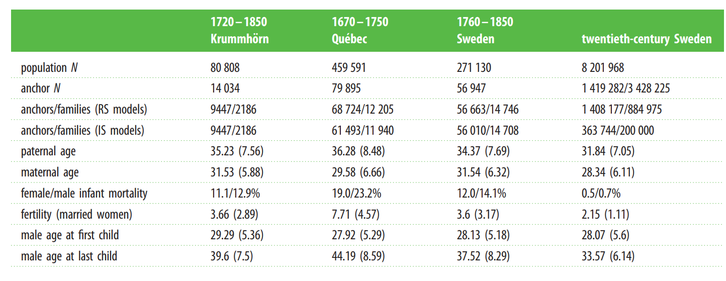
The estimates he cited were subsequently vindicated by other historians such as Eisner, and have been observed in other European countries as well:

Before we try to explain this remarkable development, let’s be sure it is real. Following the publication of Gurr’s graph, several historical criminologists dug more deeply into the history of homicide. The criminologist Manuel Eisner assembled a much larger set of estimates on homicide in England across the centuries, drawing on coroners’ inquests, court cases, and local records. Each dot on the graph in figure 3–2 is an estimate from some town or jurisdiction, plotted once again on a logarithmic scale. By the 19th century the British government was keeping annual records of homicide for the entire country, which are plotted on the graph as a gray line. Another historian, J. S. Cockburn, compiled continuous data from the town of Kent between 1560 and 1985, which Eisner superimposed on his own data as the black line.

Pinker hypothesizes that these trends have occurred due to various reasons, such as the rise of centralized states, increased rationality, and more (classically) liberal political policies. Peter Frost and Henry Harpending instead hypothesize that this decline is also driven by genetic factors, such as selection against criminality and Malthusian selection for economic status. Modeling the effect of selection for economic status on homicide rates is not possible because the genetic correlation between the social class phenotype and the criminality phenotype is unknown. Modeling the effect of executions on the other hand is easier because the correlation between the genes that cause people to murder and the genes that cause people to be executed should be close enough to perfect.

To estimate the effect of executions had on the English genome properly, some statistics must be calculated: the heritability of criminality, the age crime curve, the proportion of the population that is executed, and the mean number of children fathered by age.

Heritability of criminality

Frost argues that antisocial behaviour is highly heritable, exhibiting a heritability between .69 and .96 based on twin studies. This is accurate, but misleading. Temperament in general is highly heritable, but there is no guarantee that the individual actions that cause the use of the death penalty are based on this. Looking through a few papers that estimate the heritability of criminality based on self-reports or objective measurements, it only seems moderately heritable:

Sweden, measured (n = 1,500,000): 55%.

America, self-reported (Add Health): 0-70% depending on the model and trait.

Meta-analysis of various anti-social behaviours: 66%.

Sweden, self-reported (n = 442): 48%.

Meta-analysis of criminality, mostly based on self/family reporting: 50%.

The mean of all 5 studies and meta-analyses is 48% — a bit lower than the 69% value that Frost uses. It is possible for heritabilities to change across time, but in practice this is not observed in the real world: intelligence has always been roughly 60-90% heritable, and height has always been roughly 70-90% heritable. For the sake of simplicity, I will assume the additive and broad sense heritability are equivalent.

Age crime curve

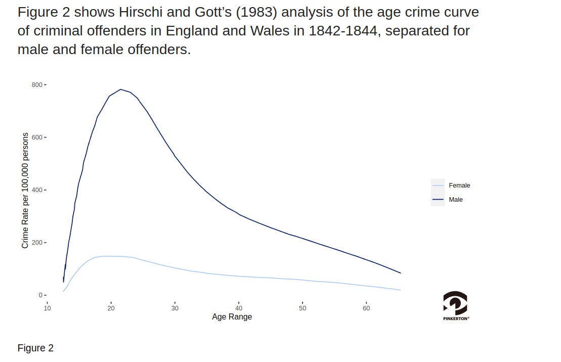
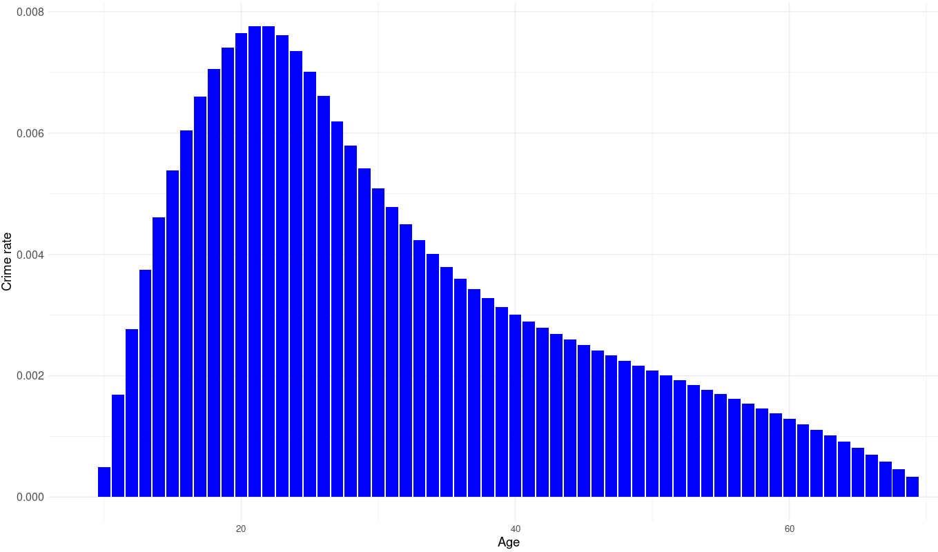
I was able to get the exact figures from this source (page 303), and interpolated the data because it was binned in age categories. Assuming some cross-temporal consistency in the age-crime curve, the relative odds of being executed by age can be computed using this data.

Fertility by age

Data on this fertility from the Middle-ages is sparse, unfortunately. Fortunately, the age at which people have children doesn’t appear to vary that much by state and time, so using modern data as a proxy should not be a problem.

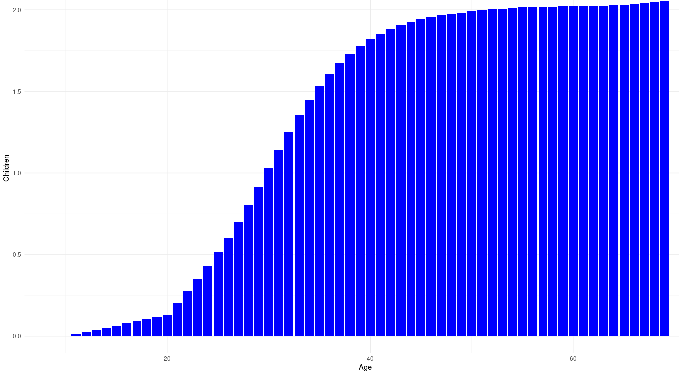
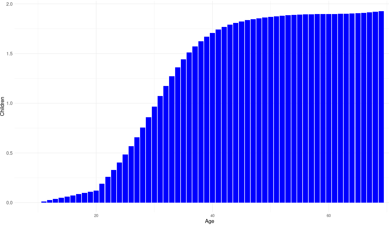
For whatever reason, getting data on fertility by age from the UK is impossible (?), so I had to use US data as a proxy instead. Controlling for cohort effects, I obtained these fertility means by age in American men from the GSS:

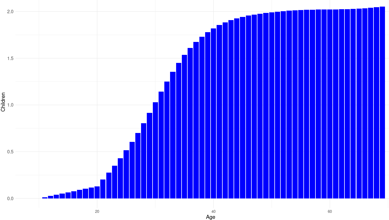
predicted values for ages 10-19 were created using a linear interpolation

It would be prudent to scale these figures to historically plausible values; the population of England was 4.73 million in 1300, and 5.2 million in 1700: an increase of 10%. Assuming a generational period of 30 years, this means that, on average, each succeeding generation had about .75% more children then the previous one [rationale : 1.0075^(400/30) = 1.1]. Taking into account that the average Brit died in this period when they were roughly 50-60 years old, they should be expected to have 2.015 surviving children at this age, so the mean number of children (adjusting for survival) should be expected to be similar to this curve:

Younger people will be expected to have more children as they get older, but this concern is irrelevant when estimating the effect of executions on evolutionary fitness. Of note is the fact that I used the age/fertility curve for men — while both men and women can be murderers and execution victims, using data for men is probably best practice, as they tend to be much more likely to be murderers regardless of the society in question.

Proportion of men that are executed

Frost and Harpending cite that, at the peak of England’s use of the death penalty, 0.5-1% of men were executed during their lifetimes, and plausibly an equal number died before execution either in prison or at the scene of the crime. They claim that support for the death penalty began in the 11th century, peaked in the 16th century, and declined substantially by the 18th century.

Change began in the 11^th century with the strengthening of kingdoms throughout Western Europe and a shift toward a new consensus. The State no longer saw itself as an honest broker in personal disputes. Jurists were now arguing that the king must punish the wicked to ensure that the good may live in peace (Carbasse, 2011, pp. 36–56). The Church was coming around to the same view:
… a reaction began to arise in the 11^th century against the previous system of monetary compensation. Henceforth, increasingly, it was felt that money could not be a sufficient compensation for such an infraction. The idea that the murder of a man is a crime too serious, an offence too manifest to the order of Creation, to be simply “compensated” by a sum of money was present from the early 11^th century onward in the thinking of some bishops. (Carbasse, 2011, pp. 37–38) [my translation]
The theologian Thomas Aquinas (1225–1274) justified the death penalty by appealing to the common good:
… it is lawful to kill an evildoer in so far as it is directed to the welfare of the whole community, so that it belongs to him alone who has charge of the community's welfare. Thus it belongs to a physician to cut off a decayed limb, when he has been entrusted with the care of the health of the whole body. Now the care of the common good is entrusted to persons of rank having public authority: wherefore they alone, and not private individuals, can lawfully put evildoers to death. [Ila Ilae, q. 64] (Aquinas, 1947)
The death penalty became not only more common but also more radical in its implementation. It was increasingly used not only for murder but also for other crimes (rape, abortion, infanticide, lèse-majesté, recurrent theft, counterfeiting, etc.). It also assumed increasingly horrendous forms: drawing and quartering, breaking on the wheel, and burning at the stake. Beginning in the 13^th and 14^th centuries, there were even cases of the convicted murderer being buried alive under the victim's casket (Carbasse, 2011, pp. 52–53).
This war on murder reached its peak in England and Flanders by the 16^th century. The courts annually put to death one person out of every ten thousand. Over a lifetime, one or two out of every two hundred men would end up being executed (Savey-Casart, 1968; Taccoen, 1982, p. 52). Others died while languishing in prison. In one medieval English jail, 25% of all inmates perished before they could be tried. By comparison, only 25% of all inmates were eventually convicted (Ireland, 1987). Although Geltner (2006) describes medieval prisons as “mostly tolerable,” he goes on to note that “the confluence of imbalanced diets, cramped quarters, and poor hygiene meant that prisoners (somewhat like monks) were particularly prone to die in epidemics, as confirmed by their decimation during the Black Death.”
[…]
By the mid-18^th century, the execution rate was falling not just because fewer murders were being committed but also because a shrinking proportion of convicted murderers were being executed. Revulsion against the death penalty was growing among judges and jurors, while people in general were for similar reasons spurning once popular events like cock fighting, bear and bull baiting, and the burning of cats on Midsummer Day (Clark, 2007, pp. 182–183; Elias, 1978, pp. 203–204). The new mood was apparent in English law courts. “Whereas in the seventeenth century a quarter of those who stood trial were hanged, this had halved by the mid-eighteenth century, and fell further by 1800” (Morgan and Rushton, 1998, p. 68). This trend resulted more from jury leniency than from actual change to the law. In the early 19^th century, for instance, hanging was still mandatory for theft of goods worth at least 40 shillings. To save a condemned man, a jury decided that a stolen 10-pound note was worth only 39 shillings. Another jury came to the same decision for a theft of 100 pounds! (Taccoen, 1982, p. 50). A similar change of mood could be observed in French law courts. In Dijon, the death penalty accounted for 13 to 14.5% of all sentences before 1750, 8.5% in 1758–1760, 6% in 1764–1766, and less than 5% after 1770 (Carbasse, 2011, p. 70). This abolition de facto was followed by abolition de jure in one European country after another from the mid-18^th century onward (Carbasse, 2011, pp. 69–75).

For the sake of simplicity, I will assume a flat execution rate of 1% for all sexes between the years 1300 and 1700.

Simple model

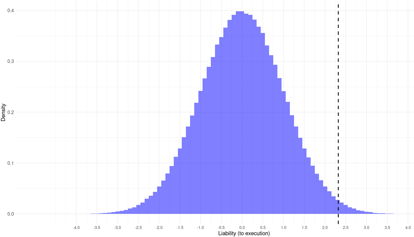
A quick explanation of the model: liability (both environmental and genetic) to being executed is normally distributed with a starting mean of 0 and standard deviation of 1 in the year 1300. Everybody who scores above 2.32 (the 99th percentile) gets executed, dies, and can no longer bear children.

Under the bell curve model, the average ‘liability to being executed’ of those who are executed is 2.65, while the liability within those who are not is -.027.

#'agg' is liability to execution, 'df' is the dataframe
mean((df %>% filter(agg > 2.32))$agg)
[1] 2.654131
mean((df %>% filter(agg < 2.32))$agg)
[1] -0.02673942

Assuming that the execution itself has no bearing on whether their children survive relative to the rest of the population, then the number of children an executed person bears can be estimated by taking the average number of expected of children weighted by the execution rate by age (which is estimated with the age-crime curve). As it’s unlikely that children under 10 will either bear children or be executed, they were ignored in the modeling process. Ages above 70 are also unmodeled.

The model estimates that the average executed individual bore about .94 surviving children, in comparison to 2.026 in those who are not executed:

#polan10$children2 is a vector which contains information of the average number of children by age
#ropz$probexe is a vector which contains the probability of being executed by age

wtd.mean(x=polan10$children2, weights = ropz$probexe)
[1] 0.937782

.01*wtd.mean(x=polan10$children2, weights = ropz$probexe)+.99*2.026
[1] 2.015118

#if 2.015 is the mean fertility of the sample, it turns out that 2.026 is the surviving fertility of those who are not executed, if the expected surviving fertility of those who are executed is .94.

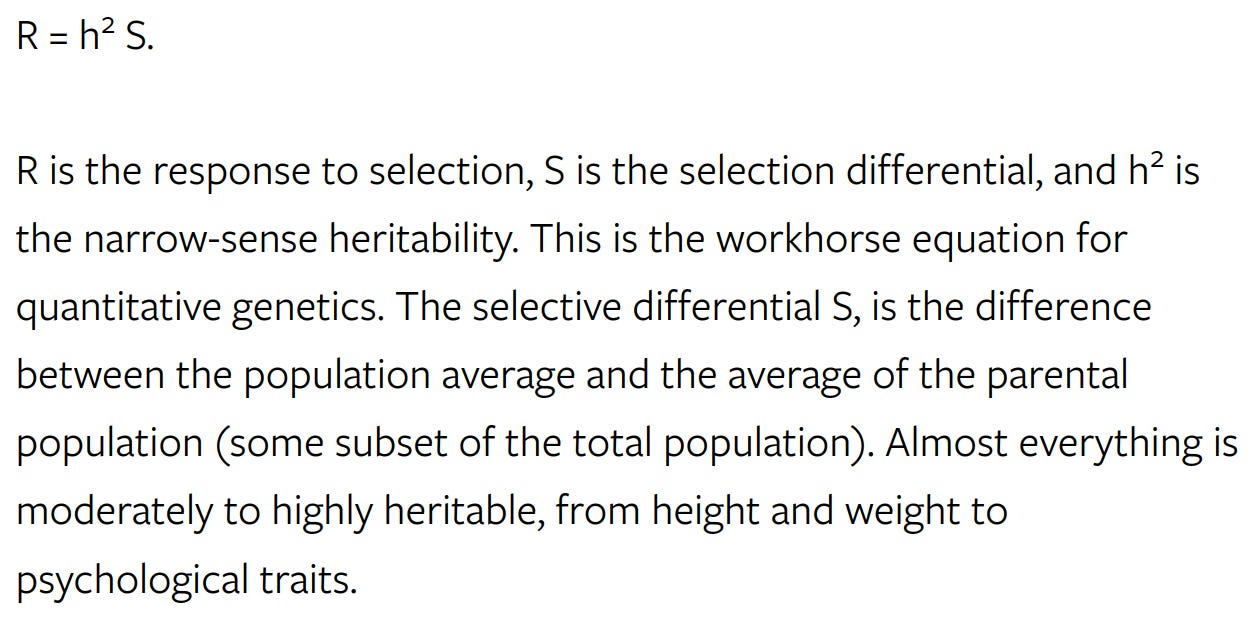
To estimate the effect this has on the next generation’s population mean in liability to being executed, the breeder’s equation was used.

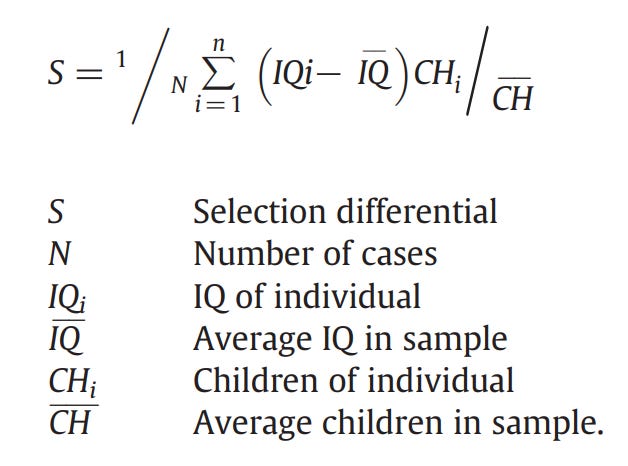
The conventional formula to compute the selection differential cannot be used because of the nature of the problem, instead, I invented a new formula for situations such as these:

Surviving fertility of group 1: sf_g1
Surviving fertility of group 2: sf_g2
Proportion of total population in group 1: p_g1
Proportion of total population in group 2: p_g2
Trait mean in group 1: tm_g1
Trait mean in group 2: tm_g2
Trait mean in the general population: TM
Trait mean within the selected population: SM
Selection differential: S


#The trait mean within the general population is calculated as follows:

TM = (p_g1 x tm_g1 + p_g2 x tm_g2)/(p_g1 + p_g2)

#The trait mean within the selected population is calculated as follows:

SM = (p_g1 x tm_g1 x sf_g1 + p_g2 x tm_g2 x sf_g2)/(p_g1 x sf_g1 + p_g2 x sf_g2)

#The selection differential, by definition, is the difference between the selected population and the general population. Meaning, that the formula would be:
S = SM - TM

Applying this formula to the current situation:

sf_g1 = wtd.mean(x=polan10$children2, weights = ropz$probexe)
sf_g2 = 2.026
p_g1 = .01
p_g2 = .99
tm_g1 = mean((df %>% filter(agg > 2.32))$agg)
tm_g2 = mean((df %>% filter(agg < 2.32))$agg)
TM = (p_g1 * tm_g1 + p_g2 * tm_g2)/(p_g1 + p_g2)
SM = (p_g1 * tm_g1 * sf_g1 + p_g2 * tm_g2 * sf_g2)/(p_g1*sf_g1 + p_g2*sf_g2)
S = SM-TM
S
[1] -0.0143592
#The selection differential is -0.0143592

Applying the breeder’s equation:

h2 <- .48
RS = S*h2
RS
[1] -0.006892416
400*RS/30
[1] -0.09189887

This means that, every generation, the liability to being executed is expected to decrease by .0069 SD. Over 400 years (1300 to 1700), this should result in a drop in liability of .092 SD.

Can this explain the drop in the homicide rate?

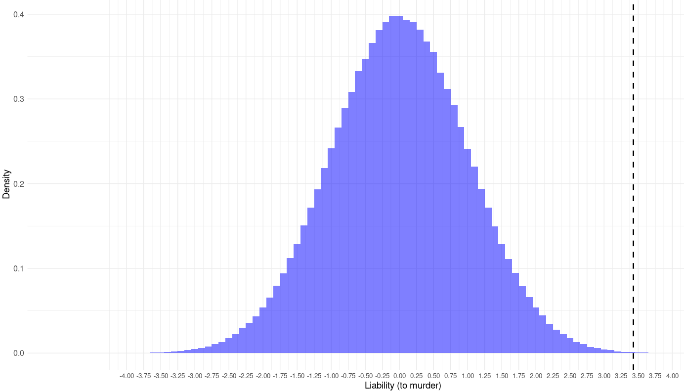
Given that the homicide rate in England was about 30 per 100,000 in the 1300s, liability to committing homicide (again, both genetic and environmental) can also be hypothesized to be gaussian with a reference mean of 0 and standard deviation of 1 in 1300. If 30 per 100,000 people committed homicide per year, then the threshold at which people commit murder is 3.43 SD above the trait mean.

Assuming that the liability to commit murder and the liability to be executed genetically correlate at 1, the selection against liability to be executed should have phenotypically reduced England’s liability to murder by the same amount (0.091 SD)

This selection effect cannot explain the reduction: a reduction of this magnitude would be expected to reduce the homicide rate from 30 to 20 per 100,000.

vec <- rnorm(100000000, mean=-0.092, sd=1)
df <- data.frame(agg = vec)
nrow((df %>% filter(agg > 3.431614)))/nrow(df)
[1] 0.000212607
nrow((df %>% filter(agg > 3.431614)))/nrow(df)*100000
[1] 21.2607
#upper line of code calculates the rate per 100,000 in a population where the trait mean is shifted leftwards by 0.092 SD

The total change in liability (assuming a drop from 30 to 2 per 100,000), according to the gaussian model, is 0.67 SD, so the selection against execution can only account for 13% of the reduction in homicide that occurred in England.

vec <- rnorm(100000000, mean=-.67, sd=1)
df <- data.frame(agg = vec)
nrow((df %>% filter(agg > 3.431614)))/nrow(df)*100000
[1] 2.09

Complex modeling

Because some of these statistics are estimated imprecisely, I have run several population models under varying assumptions to estimate how much variance there is in the percentage of the decline in homicide that can be accounted for by selection against being executed:

Homicide rate in 1300: upper bound of 40 per 100,000, lower bound of 20 per 100,000. Eisner’s figures trend closer to 20, Frost and Harpending cite figures in the 20-40 range for the late Middle ages.
Homicide rate in 1700: upper bound of 4.3 per 100,000 (rate observed in the 2nd half of the 17th Century) and lower bound of 1.4 per 100,000 (rate observed in the 2nd half of the 18th century).
Based on the preceding intervals, the smallest possible change in liability (both genetic and environmental) to commit homicide is ~.40 SD (20 per 100,000 →4.3 per 100,000) and the largest is ~.80 SD (40 per 100,000 →1.4 per 100,000). Details for this calculation are in the appendix.
Execution rate in the whole population from 1300 to 1700: Frost and Harpending claim that, at its peak, capital punishment (both formal and informal) was used against 1-2% of the male population. The rate in the general population is probably a bit more than half of that, and the overall rate, considering that the rate outside the peak will be inevitably lower. I assigned an interval of between .4% to 1%.
(additive) Heritability of criminality/execution/murder: lower bound of 36%, upper bound of 60%. I find it hard to believe that criminality is more additively heritable than intelligence (which has an additive heritability of roughly 60%), but I could believe that the additive heritability of criminality is still higher than 48% due to some unknown bias in twin modeling. 36% was assigned as the lower limit to make the interval balance around 48%.
The genetic correlation between the genes that cause people to murder and cause executions: probably pretty close to 1, but I doubt it is perfect. 0.8 was assigned the lower limit, and 1 was assigned the upper limit.
Effect of execution on the survival of children: presumably, being executed would have a negative effect on the survival of children, as it would deprive the children of a caregiver. The lowest income declile had about 2/3rds the net fertility of the 5th decile in England around this time, largely because high status children were more able to survive. Given that the children of the executed could still be reared by relatives, the effect of execution on the survival of children is probably higher than a reduction of a third, so I will set the lower limit to 1/3rd and upper limit to no effect.
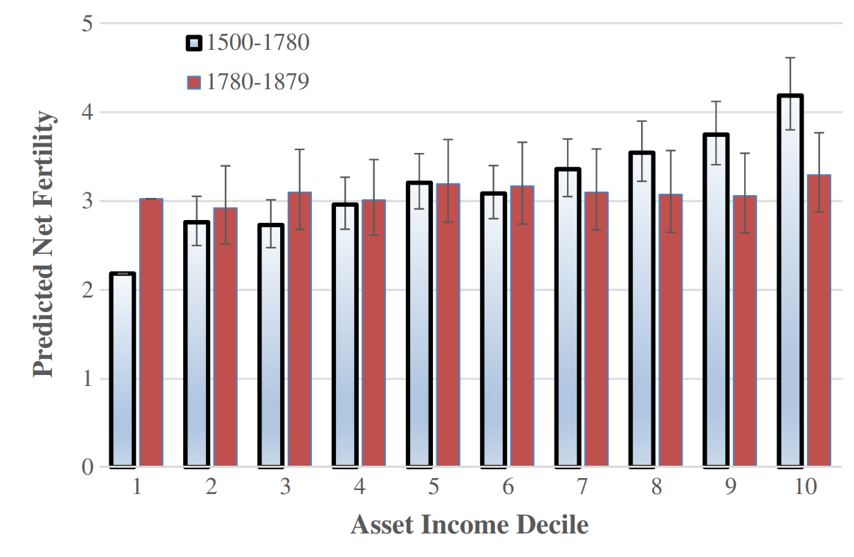
from here

Then, I made an R function that calculates the proportion of the decline that can be explained by selection against execution given a set of parameters (where the default parameters are the ones I chose in the simple model):

calculate_accounted_variance <- function(gcor=1, h2=.48, sdchange=.67, malth=1, exerate=.01) {
  tempexe <- ropz$crime*1/21*exerate/.01
  tempdf <- data.frame(agg = tempvec)
  liability_threshold <- qnorm(1-exerate)
  liability_executed <- mean((tempdf %>% filter(agg > liability_threshold))$agg)
  liability_nonexecuted <-mean((tempdf %>% filter(agg < liability_threshold))$agg)
  
  
  sf_g1 = wtd.mean(x=polan10$children2, weights = tempexe)*malth
  sf_g2 = 2.026 #assumed to be flat for simplicity's sake
  p_g1 = exerate
  p_g2 = 1-exerate
  tm_g1 = liability_executed
  tm_g2 = liability_nonexecuted
  TM = (p_g1 * tm_g1 + p_g2 * tm_g2)/(p_g1 + p_g2)
  SM = (p_g1 * tm_g1 * sf_g1 + p_g2 * tm_g2 * sf_g2)/(p_g1*sf_g1 + p_g2*sf_g2)
  S = SM-TM
  
  RS = S*h2*gcor
  phenodecline <- 400*RS/30

  return(-phenodecline/sdchange)
  
}

I then ran different combinations of these parameters to test how much adjusting these parameters changed the results, and found that tinkering with these parameters did matter quite a bit. The median model found that 11% of the decline in homicides in England from 1300 to 1700 can be explained by genetic shifts, but the fraction varies quite a bit by model, as shown by the distribution:

gcor_vec <- seq(from=.8, to=1, by=.1)
h2_vec <- seq(from=.36, to=.60, by=.08)
sdchange_vec <- seq(from=.40, to=.80, by=.10)
malth_vec <- seq(from=.60, to=1, by=.10)
exerate_vec <- seq(from=.004, to=.01, by=.002)

variance_vector <- c()

for(gc in gcor_vec) {
  for(h in h2_vec) {
    for(sd in sdchange_vec) {
      for(ma in malth_vec) {
        for(exe in exerate_vec) {
          cav <-calculate_accounted_variance(h2 = h, gcor = gc, exerate=exe, malth=ma, sdchange=sd)
          print(cav)
          variance_vector <- c(variance_vector, cav)
        }
      }
    }
  }
}

Conclusion

Unfortunately, it’s difficult to estimate how much of this decline is genetic using mathematical models, but based on the results it’s unlikely it was a large amount. And my historical knowledge of England is not deep enough to give an informed answer on whether English institutions changed enough to cause this shift in homicide rates.

Reality is very difficult to model. Because of this, I'm naturally skeptical of complex models wrt demographics, climate, and such. The problem at hand is that, no matter what assumptions are made, it is very difficult to see how executions can explain more than 20% of the decline in homicide that occurred in England during this time period.

Appendix

Code for fertility means by age (GSS):

mengss <- gss_all %>% filter(sex==1)

reg <- lm(data=mengss, childs ~ rcs(age, 8) + rcs(cohort, 8))
summary(reg)

polan <- data.frame(age=seq(from=20, to=70), children=predict.lm(lr, data.frame(age=seq(from=20, to=70), cohort=1960)))
polan
temp1 <- data.frame(age=seq(from=10, to=19), children=(seq(from=10, to=19)-10)*polan$children[1]/10)

polan10 <- rbind(temp1, polan)

ggplot(data = polan10, aes(x = age, y = children)) +
  geom_bar(stat = "identity", fill = "blue") +
  labs(title = "Average Number of Children by Age",
       x = "Age",
       y = "Children") +
  xlim(9, 70) +
  theme_minimal()

Code for the data distribution correction:

polan10$children2 <- polan10$children*2.015/1.89176798

ggplot(data = polan10, aes(x = age, y = children2)) +
  geom_bar(stat = "identity", fill = "blue") +
  labs(title = "Average Number of Children by Age",
       x = "Age",
       y = "Children") +
  xlim(9, 70) +
  theme_minimal()

Code for age interpolations:

agec <- data.frame(age = c(10, 17.5, 22.5, 27.5, 35, 45, 55, 65), crime=c((1463+1465+1423)/(2909803+2938366+2967223), (5755+5633+5146)/(793575+805586+817778), (6531+6145+5380)/(739960+756457+847932), (4008+3750+3273)/(624834+638765+578397), (4437+4058+3348)/(1020198+1040491+1061190), (2117+1935+1755)/(761076+773078+785268), (960+814+814)/(503017+509233+515525), (469+451+410)/(539606+545488+551435)))

spline_fit <- spline(agec$age, agec$crime, xout = seq(10, 65, by = 1))
spline_fit$y
ropz <- data.frame(age=seq(10, 70, by = 1), crime=spline(agec$age, agec$crime, xout = seq(10, 70, by = 1))$y)

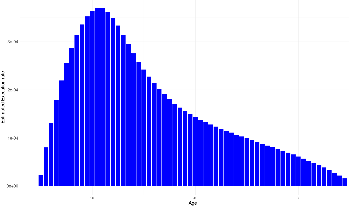
Multiplying the crime rate of each age group by 1/21 results in a 1/100 lifetime event rate:

> prod(1-ropz$crime/21)
[1] 0.9902147

Estimating the execution rate by age:

ropz$probexe <- ropz$crime/21

ggplot(data = ropz, aes(x = age, y = probexe)) +
  geom_bar(stat = "identity", fill = "blue") +
  labs(title = "",
       x = "Age",
       y = "Estimated Execution rate") +
  xlim(9, 70) +
  theme_minimal() +
  theme_bw() +
  theme_minimal() +
  theme(
    axis.text.x = element_text(size = 10),
    axis.text.y = element_text(size = 12),
    axis.title.x = element_text(size = 14),
    axis.title.y = element_text(size = 14),
    legend.position = "right",
    plot.background = element_rect(fill = "white")
  )

Maximum possible liability change estimate is about .84 SD (40 per 100,000 to 1.4 per 100,000):

vec <- rnorm(100000000, mean=0, sd=1)
df <- data.frame(agg = vec)
nrow((df %>% filter(agg > 3.352795)))/nrow(df)*100000# equals 40
[1] 39.885
vec <- rnorm(100000000, mean=-.84, sd=1)
df <- data.frame(agg = vec)
nrow((df %>% filter(agg > 3.352795)))/nrow(df)*100000# must equal 1.4
[1] 1.352

Minimum possible liability change estimate is about .38 SD (20 per 100,000 to 4.3 per 100,000):

vec <- rnorm(100000000, mean=0, sd=1)
df <- data.frame(agg = vec)
nrow((df %>% filter(agg > 3.540084)))/nrow(df)*100000
[1] 20.035
vec <- rnorm(100000000, mean=-0.38, sd=1)
df <- data.frame(agg = vec)
nrow((df %>% filter(agg > 3.540084)))/nrow(df)*100000
[1] 4.303

Code to create bell curve plot:

Fraction_of_the_decline_explained_by_selection_against_executions <- variance_vector
GG_denhist(Fraction_of_the_decline_explained_by_selection_against_executions, auto_fraction_bounary=F) +
  theme_minimal() +
  theme_bw() +
  theme(
    axis.text.x = element_text(size = 10),
    axis.text.y = element_text(size = 12),
    axis.title.x = element_text(size = 14),
    axis.title.y = element_text(size = 14),
    legend.position = "right",
    plot.background = element_rect(fill = "white")
  )

Percentiles:

> quantile(variance_vector, probs=seq(from=0, to=1, by=.05))
        0%         5%        10%        15%        20%        25%        30%        35%        40%        45%        50% 
0.03062196 0.05186102 0.06145704 0.06878992 0.07540606 0.08174463 0.08825279 0.09425791 0.10025543 0.10722047 0.11380244 
       55%        60%        65%        70%        75%        80%        85%        90%        95%       100% 
0.12044334 0.12804049 0.13687205 0.14567058 0.15538696 0.16836478 0.18365314 0.20399851 0.23439237 0.38793724

Robustness tests

Question: how consistent are the figures I calculated with other researchers?
Answer: consistent.

Frost and Harpending claim that a murder rate of 30 per 100,000 would correspond to a threshold of 3.43 SD:

In 1500, the threshold stood at 30 per 100,000 people and was 3.43 standard deviations (SD) to the right of the population mean, assuming a standard normal distribution and assuming, conservatively, that each murder was committed by a unique non-recurring murderer.

> qnorm(1-30/100000)
[1] 3.431614

Checks out.

They also claim that an execution rate of 1-2% in men corresponds to thresholds of 2.33 and 2.05 SD respectively.

the most violent 1 to 2% should form a right-hand “tail” that begins 2.33–2.05 SD to the right of the mean propensity for homicide

> qnorm(.99)
[1] 2.326348
> qnorm(.98)
[1] 2.053749
#same figures

Checks out.

They also claim that culling 1-2% of the population (assuming no reproductive success in the culled) would correspond to a selection differential of 0.027 - 0.049 SD per generation.

If we eliminate this right-hand tail and leave only the other 98–99% to survive and reproduce, we have a selection differential of 0.027 to 0.049 SD per generation.

> vec <- rnorm(100000, mean=0, sd=1)
> df <- data.frame(agg = vec)
> mean((df %>% filter(agg < 2.32))$agg)
[1] -0.02585761
> mean((df %>% filter(agg < 2.05))$agg)
[1] -0.04778395

Checks out.

Question: does the formula I developed to calculate the selection differential for dichotomous groups translate to real data?
Answer: Yes.

There are two ways to calculate selection differentials with real data: the slope/intercept formula (regress a standardized trait onto fertility using linear regression and dividing the slope by the intercept) or the complex formula that people in the population genetic community say looks clunky. But when I saw the complex formula I was able to finally intuitively understand what the statistic actually is trying to do.

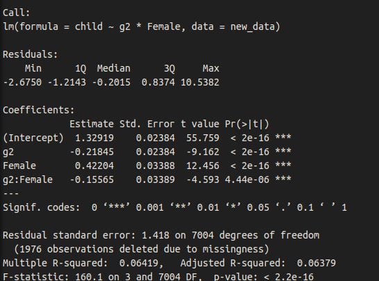
To test whether the formula works, I used real data: fertility and intelligence in the NLSY97 cohort. I dichotomized the intelligence variable to intelligent (IQ > 100) and unintelligent (IQ < 100) and restricted the sample to individuals over 35 years of age. Using the formulas I described earlier, the difference between parents and non-parents weighted by number of children is 2.48 points when intelligence is dichtomoized (It’s 2.88 when it is a continuous variable).

#g2 is IQ normalized to a mean of 0 and standard deviation of 1 within genders
new_data$intelligent <- NA
new_data$intelligent[new_data$g2 < 0] <- 0
new_data$intelligent[new_data$g2 > 0] <- 1

#this is the result of using the complex formula
selectdiffsd(iq=new_data$intelligent, kid=new_data$child)[2]*15
   estimate
1 -2.484395
#this is the result of using the slope/intercept formula
selectdiffsd2(iq=new_data$intelligent, kid=new_data$child)[2]*15
   estimate
1 -2.484949
#the disparity is probably due to computational errors.

Using the formula I developed:


intelligent <- new_data %>% filter(intelligent==1 & !is.na(child))
unintelligent <- new_data %>% filter(intelligent==0 & !is.na(child))
new_data %>% group_by(intelligent) %>% summarise(n = n())
# A tibble: 3 × 2
  intelligent     n
        <dbl> <int>
1           0  3334
2           1  3674
3          NA  1976

sf_g1 = mean(intelligent$child, na.rm=T)
sf_g2 = mean(unintelligent$child, na.rm=T)
p_g1 = nrow(intelligent)/(nrow(intelligent) + nrow(unintelligent))
p_g2 = nrow(unintelligent)/(nrow(intelligent) + nrow(unintelligent))
tm_g1 = 1
tm_g2 = 0
TM = (p_g1 * tm_g1 + p_g2 * tm_g2)/(p_g1 + p_g2)
SM = (p_g1 * tm_g1 * sf_g1 + p_g2 * tm_g2 * sf_g2)/(p_g1*sf_g1 + p_g2*sf_g2)
S = SM-TM

#divide by the standard deviation to get the change in the phenotype in SDs
S/sd(new_data$intelligent,na.rm=T)*15
[1] -2.490863
selectdiffsd(iq=new_data$intelligent, kid=new_data$child)[2]*15
   estimate
1 -2.490863
selectdiffsd2(iq=new_data$intelligent, kid=new_data$child)[2]*15
   estimate
1 -2.491218

It also works for other phenotypes, such as educational attainment (dichotomized as below associates and associates and above):

new_data$educated <- NA
new_data$educated[new_data$Z9083900 < 3] <- 0
new_data$educated[new_data$Z9083900 > 2] <- 1

educated <- new_data %>% filter(educated==1 & !is.na(child))
uneducated <- new_data %>% filter(educated==0 & !is.na(child))

new_data %>% group_by(educated) %>% summarise(n = n())
# A tibble: 3 × 2
  educated     n
     <dbl> <int>
1        0  5666
2        1  3287
3       NA    31

sf_g1 = mean(educated$child, na.rm=T)
sf_g2 = mean(uneducated$child, na.rm=T)
p_g1 = nrow(educated)/(nrow(uneducated) + nrow(educated))
p_g2 = nrow(uneducated)/(nrow(uneducated) + nrow(educated))
tm_g1 = 1
tm_g2 = 0
TM = (p_g1 * tm_g1 + p_g2 * tm_g2)/(p_g1 + p_g2)
SM = (p_g1 * tm_g1 * sf_g1 + p_g2 * tm_g2 * sf_g2)/(p_g1*sf_g1 + p_g2*sf_g2)
S = SM-TM

S/sd(new_data$educated,na.rm=T)
[1] -0.09718907
selectdiffsd(iq=new_data$educated, kid=new_data$child)[2]
     estimate
1 -0.09718907
selectdiffsd2(iq=new_data$educated, kid=new_data$child)[2]
     estimate
1 -0.09719992

Other analyses

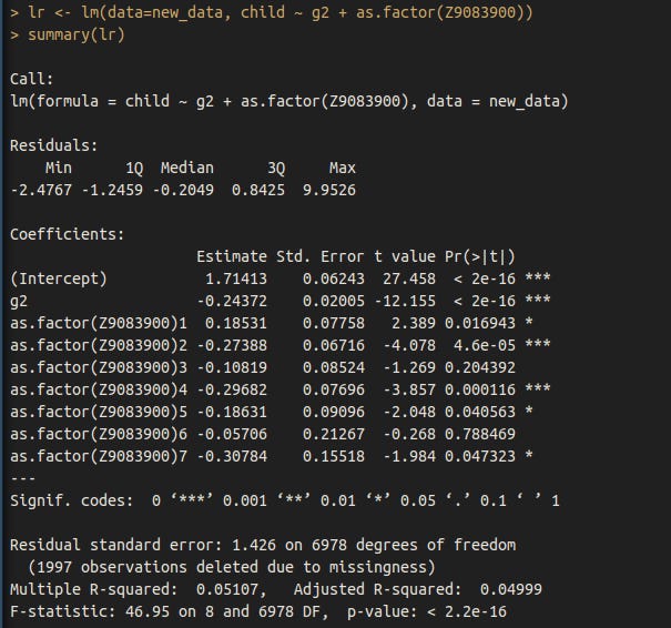
Dysgenics for intelligence are stronger in women.

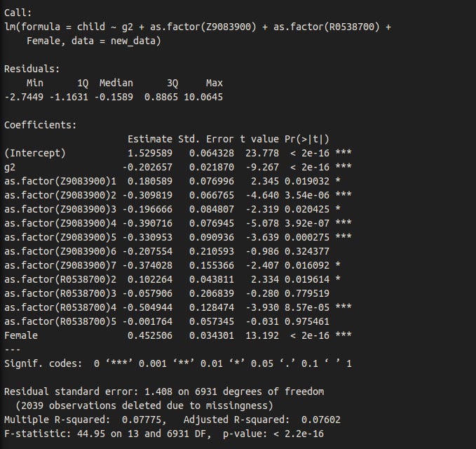
The relationship between IQ and fertility remains after controlling for education.

And race + sex.

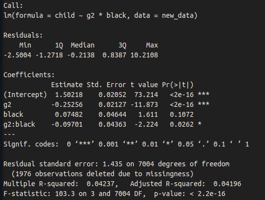
Dysgenic fertility for intelligence is stronger in Blacks than those of other races, though the p-value is not great. For what it is worth, Meisenberg found the same result in his analysis of the NLSY79.

Formulas to calculate selection differentials

selectdiffsd <- function(iq, kid) {
  d <- data.frame(iq, kid)
  d <- na.omit(d)
  d$iq <- normalise(d$iq)
  parameter <- 0
  estimate <- 0
  daf <- data.frame(parameter, estimate)
  daf$parameter <- nrow(d)-2
  daf$estimate <- 1/nrow(d)*sum((d$iq-mean(d$iq, na.rm=T))*d$kid, na.rm=T)/mean(d$kid, na.rm=T)
  return(daf)
}

selectdiffsd2 <- function(iq, kid) {
  d <- data.frame(iq, kid)
  d <- na.omit(d)
  d$iq <- normalise(d$iq)
  parameter <- 0
  estimate <- 0
  daf <- data.frame(parameter, estimate)

  if(nrow(d) > 0) {
    lr <- lm(data=d, kid ~ iq)

    daf$parameter <- nrow(d)-2
    daf$estimate <- lr$coefficients[2]/lr$coefficients[1]
  }
  else {
    daf$parameter <- NA
    daf$estimate <- NA
  }