Is Intelligence Really Normally Distributed? Part 2

I posted on this topic a few months ago, concluding that most batteries of IQ tests follow a left-tailed distribution, such as the Project Talent (PT) battery.

Some commenters related this finding to Spearman’s Law of Diminishing Returns (SLODR), the observation that subtest correlations are higher in lower ability samples. Most tests of the theory suggest that it is true, though some suggest that it is not or that the effect is more complicated than previously thought. Independent of whether the effect exists, a left-tailed distribution of intelligence would be a more likely observation in a universe where SLODR is true, but the observations are not inter-dependent.

If g followed a left-skewed distribution, and the non-g residuals of intelligence were normally distributed, then it is likely that SLODR would hold. However, if the non-g residuals are also skewed, then the question becomes much more complicated. The correlations between subtests could also vary by ability level for reasons beyond artefacts of the distribution.

There is also the question of the threshold hypothesis; there are multiple variants of this theory, but the most commonly cited one is that IQ does not matter past 120, which is not empirically validated.

There is also the issue that IQ tests do not actually measure intelligence, rather, they measures differences between individuals in performance on a given battery of cognitive tests. The latter highly correlates with the former, but there is no guarantee that these distributions are identical, as IQ is measured and on an interval scale, and intelligence is a property of the world and is on a ratio scale (e.g. a rock has no intelligence, but not an IQ of 0).

The post was also criticized on the grounds that it did not take into consideration ceiling (or floor) effects in the subtests. To test whether these biases mattered, I:

• Took the Project Talent dataset, and subset the sample to 14-18 year old non-Jewish white men.

• Adjusted every subtest in the PT for age.

• Measured the ceiling and floor of each subtest.

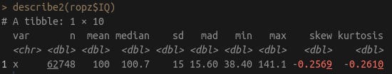
• Simulated 63k people with normally distributed g values.

• Simulated normally distributed clones of each of the PT subtests, where their g-loadings imitated those observed on the real test, and set the ceilings/floors to those that were observed empirically.

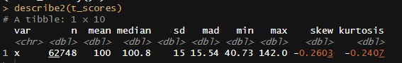
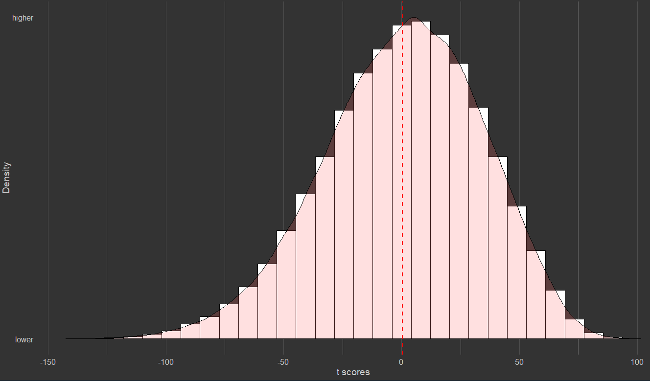
The simulated scores were only slightly skewed (-0.03), indicating that the floors and ceilings had little to do with the skewness that was observed in real data.

IQ is the simulated IQ scores, g is the simulated latent intelligence. On the real PT battery, scores had a skewness and kurtosis of -0.26.

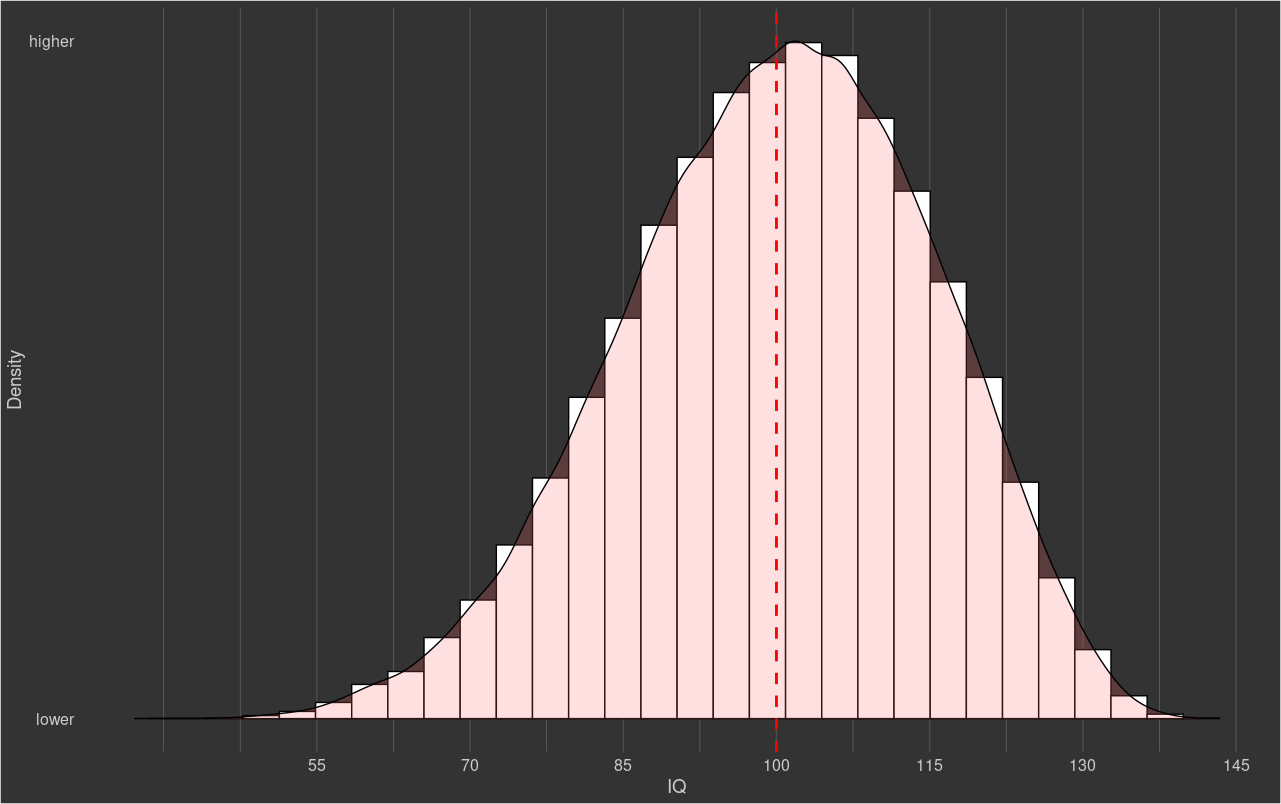
Although nobody mentioned this on twitter or in the comments section, the distribution of intelligence could also be an artefact of how the IQ scores were computed; as such, I scored the PT sample using every calculation method that came to mind. As in the previous exercise, I subest the data to non-Jewish white men between the ages of 14 and 18 and adjust the (individual) subtests for age.

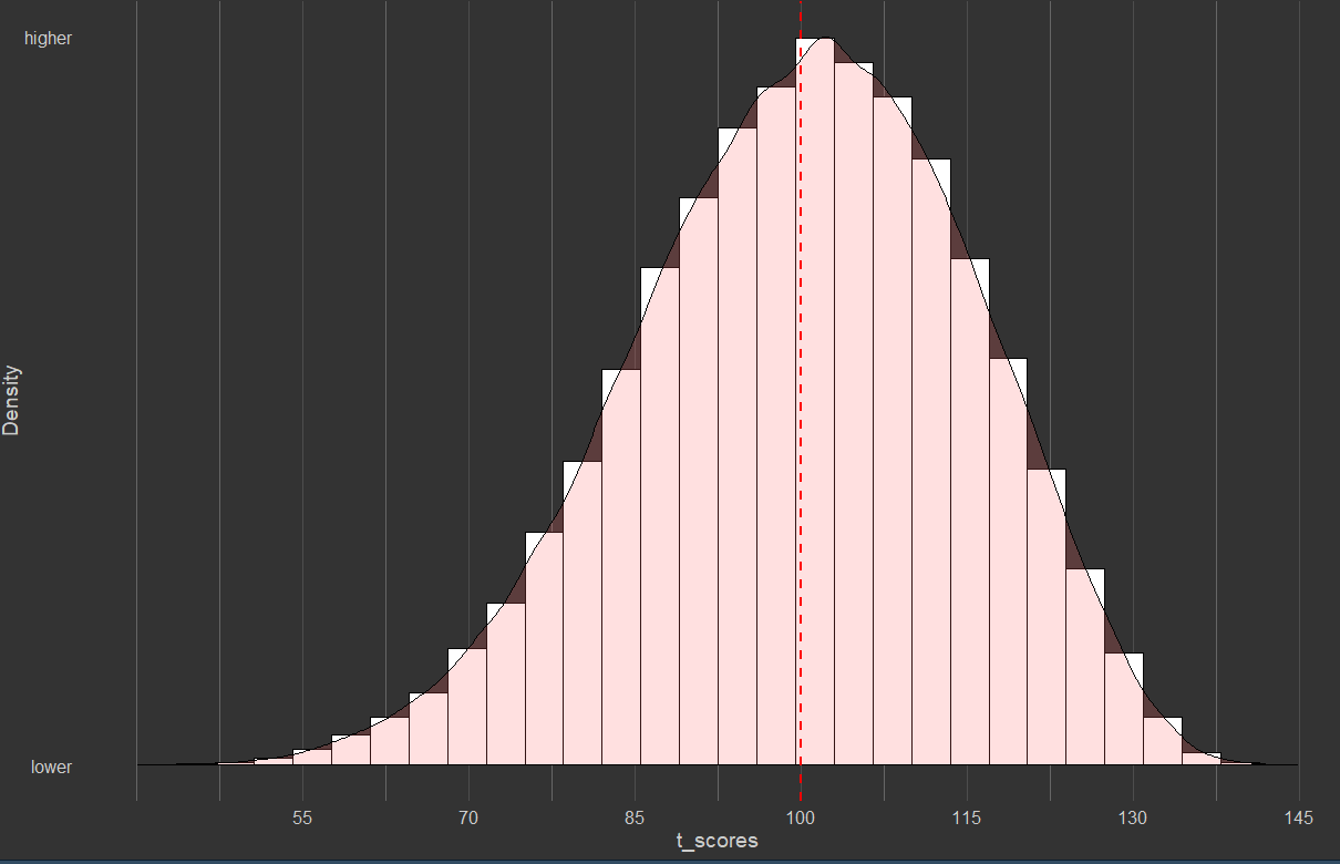
Principal component analysis (original method)

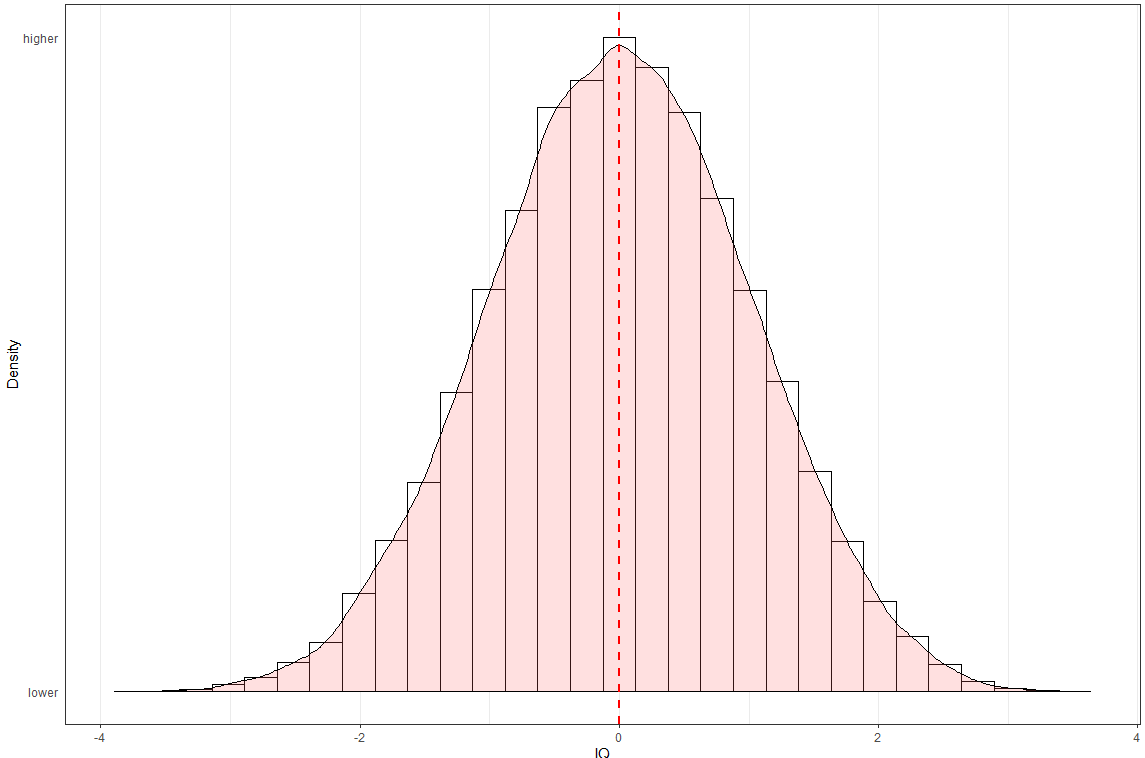
Factor analysis

Slightly more skew and less kurtosis.

Addition (e.g. score = subtest_1 + subtest_2 + …)

Higher skewness and kurtosis.

not normed to 100/15

Principal components analysis (first factor of 10, varimax rotation)

Less skewness and kurtosis, higher maximum.

Factor analysis (first factor of 10, varimax rotation)

Less skewness and kurtosis, higher maximum.

note - SD = 14

Final thoughts

Every single method used to calculate IQ scores resulted in a left-tailed distribution, though it’s not clear whether intelligence itself does; my suspicion is that the distributions for both traits are roughly the same, though I have no proof this is the case, and do not think that this proof will ever come to light.

Code for ceilings/floors analysis

#getcolindex returns the column index
#getpc extracts the first principal component
#GG_scatter plots a regression
#agecorrect corrects for age

#cleaning
data$sub = as.numeric(data$BY_SEX)
data$Female = data$sub

data$sub = as.numeric(data$BY_AGEEST)
data$BY_AGEEST
data$is99 = (data$sub/100 - floor(data$sub/100))*100
data$age60 = (data$sub/100 - floor(data$sub/100))*100/12 + as.integer(data$sub)/100 - (data$sub/100 - floor(data$sub/100))
data$age60[data$is99 == 99] <- NA
data$age60[data$BY_AGEEST==""] <- NA
data$age60[data$age60>30] <- NA
data$age60[data$age60<9] <- NA

GG_denhist(data, 'age60')
cor.test(data$age60, data$sub, method='spearman')
data$race <- as.factor(as.numeric(data$BY_RACE))

nd <- data
##########cognitive scoring
getcolindex('BY_R101', nd)
getcolindex('BY_R440', nd)
getcolindex('BY_R162', nd)
getcolindex('BY_R150a', nd)
getcolindex('BY_R150b', nd)
getcolindex('BY_R190', nd)
getcolindex('BY_R192', nd)
getcolindex('BY_F410', nd)
getcolindex('BY_F440', nd)
getcolindex('BY_F410', nd)
getcolindex('BY_F430', nd)

for(i in 63:144) {
  nd[, i] <- as.numeric(unlist(nd[, i]))
  nd[, i][nd[, i] == -999] <- NA
  if(i < 133 | i > 136) {
    nd[, i][nd[, i] == -9] <- NA
  }
  if(!i==133 & !i == 135) {
    nd[, i][nd[, i] == -99] <- NA
  }}

nd <- nd[, -getcolindex('BY_R172', nd)]
print('l')
nd <- nd[, -getcolindex('BY_R100', nd)]
print('l')
nd <- nd[, -getcolindex('BY_R320', nd)]
print('l')
nd <- nd[, -getcolindex('BY_R334', nd)]
print('l')
nd <- nd[, -getcolindex('BY_R190', nd)]
print('l')
nd <- nd[, -getcolindex('BY_R230', nd)]
print('l')
nd <- nd[, -getcolindex('BY_R340', nd)]
print('l')

getcolindex('BY_R102', nd)
getcolindex('BY_R162', nd)
getcolindex('BY_R150a', nd)
nd <- nd[, -getcolindex('BY_R150a', nd)]
getcolindex('BY_R150b', nd)
nd <- nd[, -getcolindex('BY_R150b', nd)]
getcolindex('BY_R149', nd)
nd$BY_R

nd$arithfast <- nd$BY_F410
nd$table <- nd$BY_F420
nd$cler <- nd$BY_F430
nd$obj <- nd$BY_F440
nd$spell = nd$BY_R231
nd$capital = nd$BY_R232
nd$punct = nd$BY_R233
nd$english = nd$BY_R234
nd$express = nd$BY_R235
nd$sentmemory = nd$BY_R211
nd$wordmemory = nd$BY_R212
nd$disgwords = nd$BY_R220
nd$words = nd$BY_R240
nd$reading = nd$BY_R250
nd$create = nd$BY_R260
nd$mech = nd$BY_R270
nd$twod = nd$BY_R281
nd$threed = nd$BY_R282
nd$abst = nd$BY_R290
nd$arith = nd$BY_R311
nd$bmath = nd$BY_R312
nd$amath = nd$BY_R333
nd$screening = nd$BY_R101
nd$vock = nd$BY_R102 + nd$BY_R162
nd$litk = nd$BY_R103
nd$musk = nd$BY_R104
nd$sstudiesk = nd$BY_R105
nd$mathk = nd$BY_R106
nd$phsk = nd$BY_R107
nd$biok = nd$BY_R108
nd$sciattk = nd$BY_R109
nd$aerok = nd$BY_R110
nd$eleck = nd$BY_R111
nd$mechk = nd$BY_R112
nd$farmk = nd$BY_R113
nd$homek = nd$BY_R114
nd$sportk = nd$BY_R115
nd$artk = nd$BY_R131
nd$lawk = nd$BY_R132
nd$healthk = nd$BY_R133
nd$engk = nd$BY_R134
nd$archk = nd$BY_R135
nd$jourk = nd$BY_R136
nd$fork = nd$BY_R137
nd$militk = nd$BY_R138
nd$salesk = nd$BY_R139
nd$prack = nd$BY_R140
nd$clerick = nd$BY_R141
nd$biblek = nd$BY_R142
nd$colorsk = nd$BY_R143
nd$etiqk = nd$BY_R144
nd$huntk = nd$BY_R145
nd$fishk = nd$BY_R146
nd$outdk = nd$BY_R147
nd$photok = nd$BY_R148
nd$gamesk = nd$BY_R149
nd$theatk = nd$BY_R150
nd$foodk = nd$BY_R151
nd$misc = nd$BY_R152

deeef <- subset(nd, !is.na(nd$age60))
unique(deeef$age60)
deeef$race <- ""
deeef$race[deeef$BY_RACE=='1'] <- 'White'
deeef$race[deeef$Y5_P111=='3'] <- 'Jewish'
deeef$race[deeef$BY_RACE=='2'] <- 'Black'
deeef$race[deeef$BY_RACE=='3'] <- 'Asian'
deeef$race[deeef$BY_RACE=='4'] <- 'Amerindian'
deeef$race[deeef$BY_RACE=='5'] <- 'Hispanic'
deeef$race[deeef$BY_RACE=='6'] <- 'Hispanic'
deeef$race[deeef$BY_RACE=='7'] <- 'Amerindian'
deeef$race[deeef$BY_RACE=='8'] <- 'Hispanic'
deeef$race[deeef$Y5_P111=='3'] <- 'Jewish'

deeef <- deeef %>% filter(age60 > 14 & age60<18.99)
deeef <- deeef %>% filter(Female==1)
deeef <- deeef %>% filter(race=='White')

deeef$g2  = getpc(deeef[, 2101:2159], normalizeit=T, dofa=F, fillmissing=F)*15+100
describe2(deeef$g2)
plot.new()


c <- (max(deeef$g2, na.rm=T) - mean(deeef$g2, na.rm=T))/sd(deeef$g2, na.rm=T)
c

for(i in 2101:2159) {
  deeef$subit <- as.numeric(unlist(deeef[, i]))  # Corrected this line to properly convert to numeric
  deeef[!is.na(deeef$subit), i] <- agecorrect('subit', 'age60', normalizeit=T, datafr=deeef, splinex=6)
}

ceiling <- rep(NA, 59)
floor <- rep(NA, 59)
for(i in 1:59) {
  ceiling[i] <- (max(deeef[, i+2100] %>% unlist(), na.rm=T) - mean(deeef[, i+2100] %>% unlist(), na.rm=T))/sd(deeef[, i+2100] %>% unlist(), na.rm=T)
  floor[i] <- (min(deeef[, i+2100] %>% unlist(), na.rm=T) - mean(deeef[, i+2100] %>% unlist(), na.rm=T))/sd(deeef[, i+2100] %>% unlist(), na.rm=T)
}
ceiling
floor
median(ceiling)

pc <- pca(deeef[, 2101:2159])
pc$loadings

subtests <- data.frame(ceilings = ceiling, floors=floor, gloads = pc$loadings)
subtests$names <- colnames(deeef[, 2101:2159])
GG_scatter(subtests, 'gloads', 'floors', case_names='names')

set.seed(123)
g <- rnorm(63000, mean=0, sd=1)

subby <- pmin(g, 3) 

subtest_data <- data.frame(g = g)

for (i in 1:nrow(subtests)) {
  subtest <- g * subtests$gloads[i] +  rnorm(63000, mean=0, sd=1)*sqrt(1-subtests$gloads[i]^2)
  subtest <- pmin(subtest, subtests$ceilings[i]) 
  subtest <- pmax(subtest, subtests$floors[i]) 
  subtest_data[[paste0("var_", i)]] <- subtest
}

subtest_data$IQ  = getpc(subtest_data[, 1:59], normalizeit=T, dofa=F, fillmissing=F)

cor.test(subtest_data$IQ, subtest_data$g)

describe2(subtest_data$IQ)
describe2(subtest_data$g)

Other news

• I fainted twice (almost thrice) on April 21st. I assumed that the first faint was a seizure because I saw my legs convulse 2 seconds before I blacked out, but I had no idea that fainting could also lead to convlusions. When I woke up, I went to knock on my neighbour’s door for help, though they were not there. I passed out again, and woke up a few feet from their doormat. Another neighbour saw me passed out, and I woke up around the time he noticed me on the floor. He watched over me for a few minutes; after I told him that I hadn’t taken any drugs and that I took the COVID vaccine, he attributed the events to it. The episodes were probably caused by low blood glucose, and I fully recovered a few hours later.

• I’ve been less active lately; I still plan to write, but I’m thinking of pivoting into visual content, with the first videos being explanations of twin/adoption/pedigree studies, intelligence/IQ, genes/race, etc. Kind of like what the alt hype did back in the day, but better.

• I am in the process of rewriting blog posts on The Anime Elitist and sebjenseb. Some of it is because I tend to make random errors, but what prompted me to do this was that I was starting to forget things that I had already written about.